High-Level Computer Vision n Detection of classes of

High-Level Computer Vision n Detection of classes of objects (faces, motorbikes, trees, cheetahs) in images n Recognition of specific objects such as George Bush or machine part #45732 n Classification of images or parts of images for medical or scientific applications n Recognition of events in surveillance videos n Measurement of distances for robotics 1

High-level vision uses techniques from AI. n Graph-Matching: A*, Constraint Satisfaction, Branch and Bound Search, Simulated Annealing n Learning Methodologies: Decision Trees, Neural Nets, SVMs, EM Classifier n Probabilistic Reasoning, Belief Propagation, Graphical Models 2

Graph Matching for Object Recognition n For each specific object, we have a geometric model. n The geometric model leads to a symbolic model in terms of image features and their spatial relationships. n An image is represented by all of its features and their spatial relationships. n This leads to a graph matching problem. 3

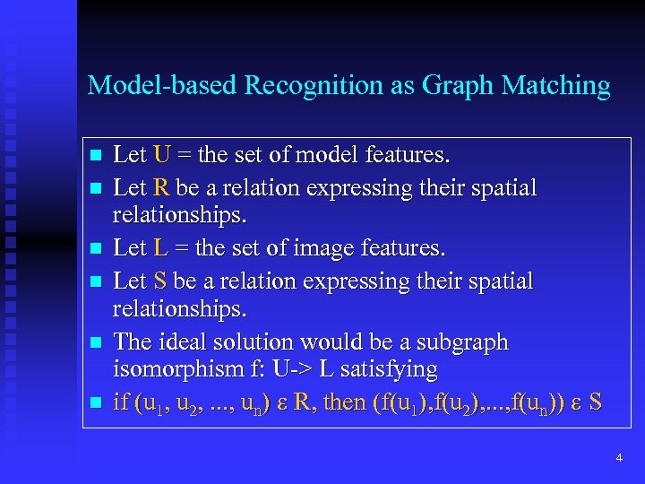Model-based Recognition as Graph Matching n n n Let U = the set of model features. Let R be a relation expressing their spatial relationships. Let L = the set of image features. Let S be a relation expressing their spatial relationships. The ideal solution would be a subgraph isomorphism f: U-> L satisfying if (u 1, u 2, . . . , un) R, then (f(u 1), f(u 2), . . . , f(un)) S 4

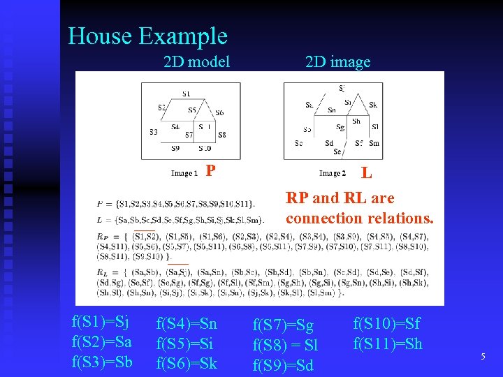House Example 2 D model P f(S 1)=Sj f(S 2)=Sa f(S 3)=Sb f(S 4)=Sn f(S 5)=Si f(S 6)=Sk 2 D image L RP and RL are connection relations. f(S 7)=Sg f(S 8) = Sl f(S 9)=Sd f(S 10)=Sf f(S 11)=Sh 5

But this is too simplistic n The model specifies all the features of the object that may appear in the image. n Some of them don’t appear at all, due to occlusion or failures at low or mid level. n Some of them are broken and not recognized. n Some of them are distorted. n Relationships don’t all hold. 6

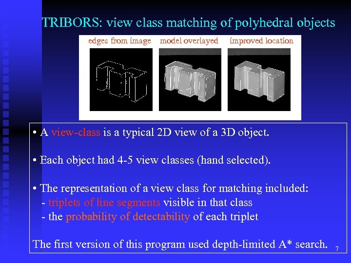TRIBORS: view class matching of polyhedral objects edges from image model overlayed improved location • A view-class is a typical 2 D view of a 3 D object. • Each object had 4 -5 view classes (hand selected). • The representation of a view class for matching included: - triplets of line segments visible in that class - the probability of detectability of each triplet The first version of this program used depth-limited A* search. 7

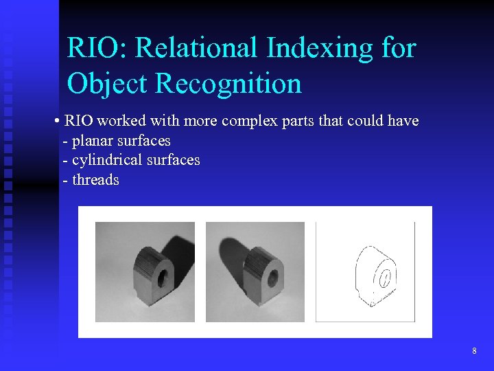RIO: Relational Indexing for Object Recognition • RIO worked with more complex parts that could have - planar surfaces - cylindrical surfaces - threads 8

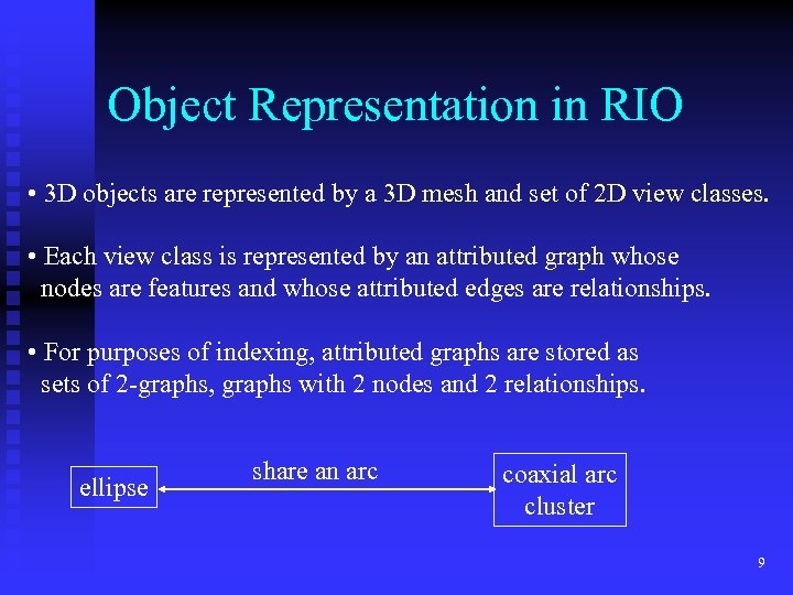Object Representation in RIO • 3 D objects are represented by a 3 D mesh and set of 2 D view classes. • Each view class is represented by an attributed graph whose nodes are features and whose attributed edges are relationships. • For purposes of indexing, attributed graphs are stored as sets of 2 -graphs, graphs with 2 nodes and 2 relationships. ellipse share an arc coaxial arc cluster 9

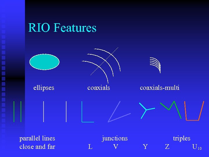RIO Features ellipses parallel lines close and far coaxials L junctions V coaxials-multi triples Y Z U 10

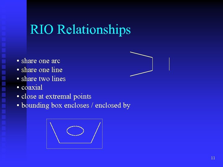RIO Relationships • share one arc • share one line • share two lines • coaxial • close at extremal points • bounding box encloses / enclosed by 11

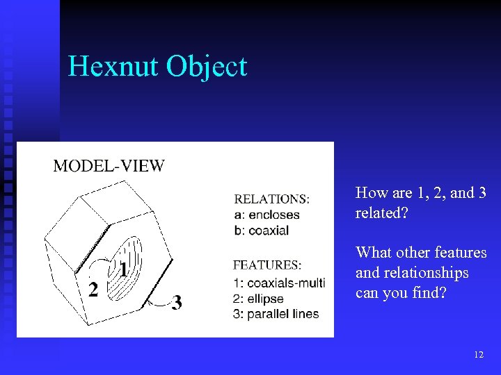Hexnut Object How are 1, 2, and 3 related? What other features and relationships can you find? 12

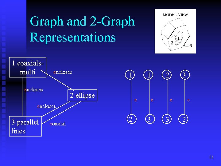Graph and 2 -Graph Representations 1 coaxialsmulti encloses 1 2 ellipse 1 e 2 e 3 e c encloses 3 parallel lines coaxial 2 3 3 2 13

Relational Indexing for Recognition Preprocessing (off-line) Phase for each model view Mi in the database • encode each 2 -graph of Mi to produce an index • store Mi and associated information in the indexed bin of a hash table H 14

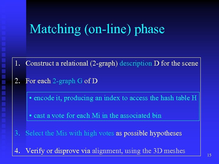Matching (on-line) phase 1. Construct a relational (2 -graph) description D for the scene 2. For each 2 -graph G of D • encode it, producing an index to access the hash table H • cast a vote for each Mi in the associated bin 3. Select the Mis with high votes as possible hypotheses 4. Verify or disprove via alignment, using the 3 D meshes 15

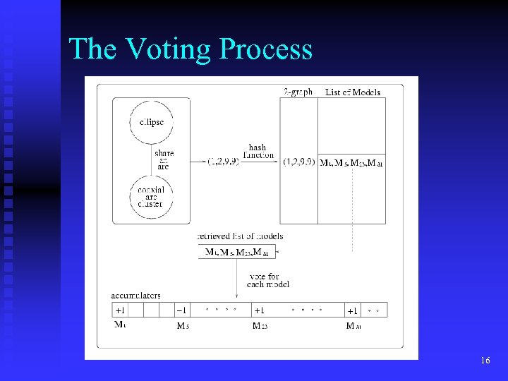The Voting Process 16

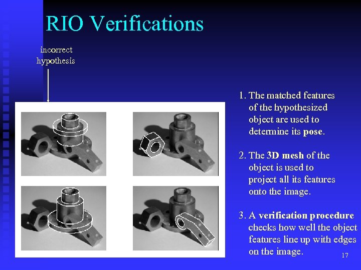RIO Verifications incorrect hypothesis 1. The matched features of the hypothesized object are used to determine its pose. 2. The 3 D mesh of the object is used to project all its features onto the image. 3. A verification procedure checks how well the object features line up with edges on the image. 17

Use of classifiers is big in computer vision today. n 2 Examples: u u Rowley’s Face Detection using neural nets Our 3 D object classification using SVMs 18

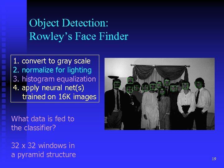Object Detection: Rowley’s Face Finder 1. 2. 3. 4. convert to gray scale normalize for lighting histogram equalization apply neural net(s) trained on 16 K images What data is fed to the classifier? 32 x 32 windows in a pyramid structure 19

3 D-3 D Alignment of Mesh Models to Mesh Data • Older Work: match 3 D features such as 3 D edges and junctions or surface patches • More Recent Work: match surface signatures - curvature at a point - curvature histogram in the neighborhood of a point - Medioni’s splashes * - Johnson and Hebert’s spin images 20

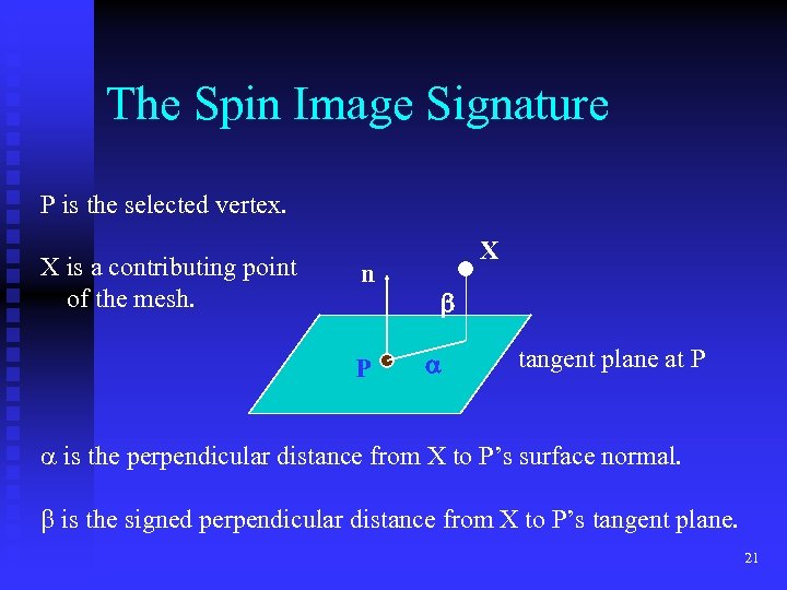The Spin Image Signature P is the selected vertex. X is a contributing point of the mesh. n P X tangent plane at P is the perpendicular distance from X to P’s surface normal. is the signed perpendicular distance from X to P’s tangent plane. 21

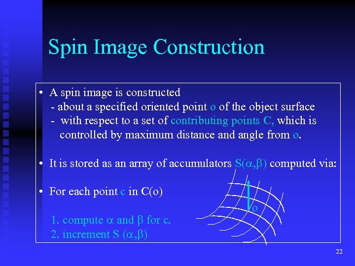Spin Image Construction • A spin image is constructed - about a specified oriented point o of the object surface - with respect to a set of contributing points C, which is controlled by maximum distance and angle from o. • It is stored as an array of accumulators S( , ) computed via: • For each point c in C(o) 1. compute and for c. 2. increment S ( , ) o 22

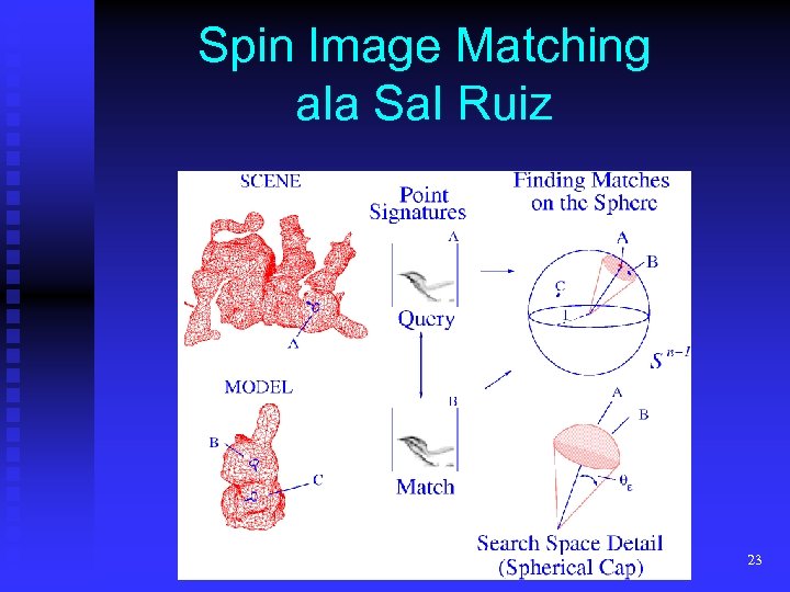Spin Image Matching ala Sal Ruiz 23

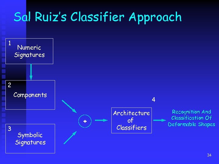Sal Ruiz’s Classifier Approach 1 Numeric Signatures 2 Components 3 4 + Symbolic Signatures Architecture of Classifiers Recognition And Classification Of Deformable Shapes 24

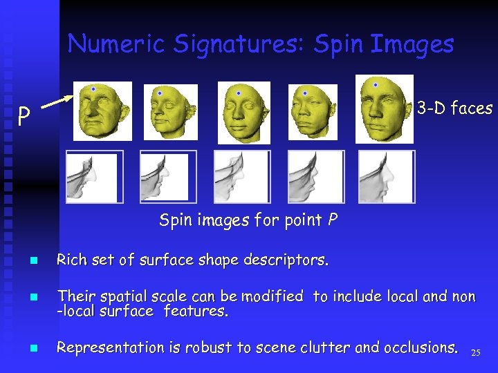Numeric Signatures: Spin Images 3 -D faces P Spin images for point P n Rich set of surface shape descriptors. n Their spatial scale can be modified to include local and non -local surface features. n Representation is robust to scene clutter and occlusions. 25

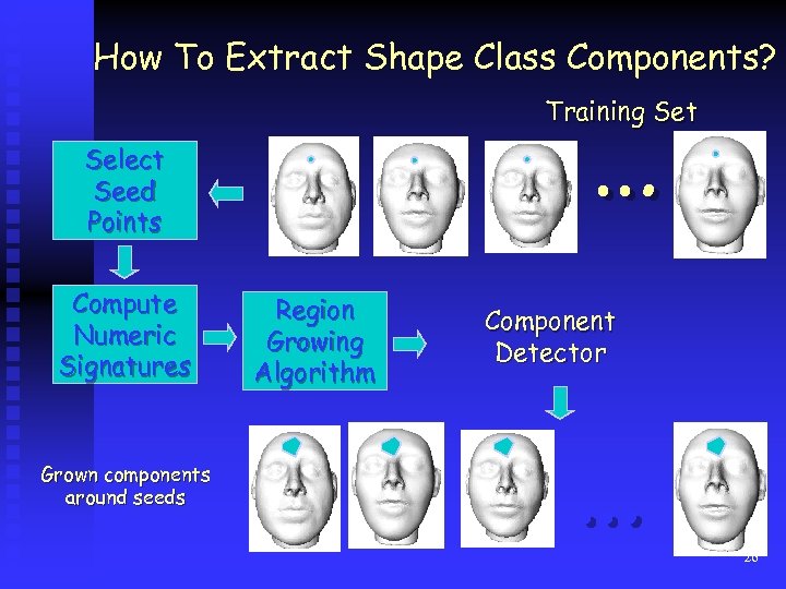How To Extract Shape Class Components? … Training Set Select Seed Points Compute Numeric Signatures Grown components around seeds Region Growing Algorithm Component Detector … 26

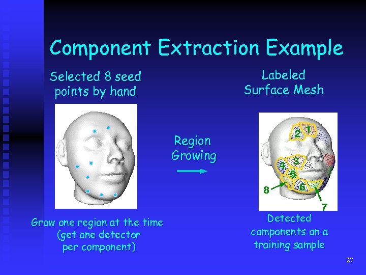Component Extraction Example Labeled Surface Mesh Selected 8 seed points by hand Region Growing Grow one region at the time (get one detector per component) Detected components on a training sample 27

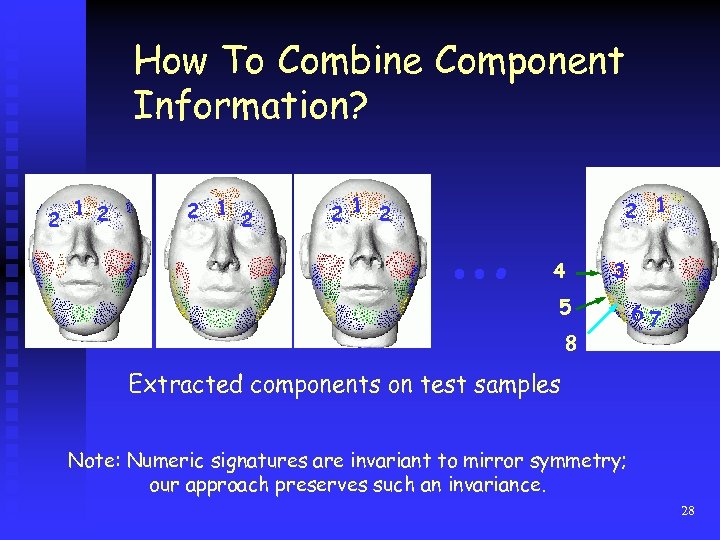How To Combine Component Information? 1 2 2 2 1 2 21 2 … 2 1 4 3 5 8 67 Extracted components on test samples Note: Numeric signatures are invariant to mirror symmetry; our approach preserves such an invariance. 28

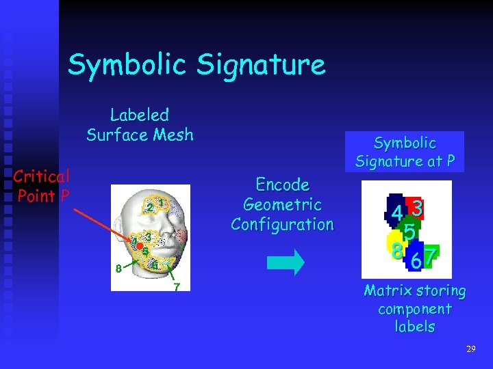Symbolic Signature Labeled Surface Mesh Critical Point P Symbolic Signature at P Encode Geometric Configuration 43 5 8 67 Matrix storing component labels 29

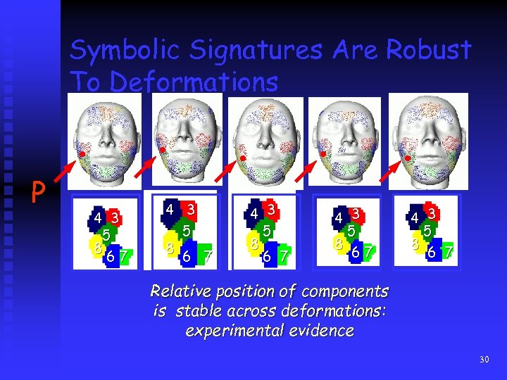Symbolic Signatures Are Robust To Deformations P 4 3 5 8 67 4 3 5 8 6 7 Relative position of components is stable across deformations: experimental evidence 30

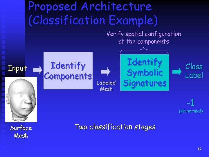Proposed Architecture (Classification Example) Verify spatial configuration of the components Input Identify Components Labeled Mesh Identify Symbolic Signatures Class Label -1 (Abnormal) Surface Mesh Two classification stages 31

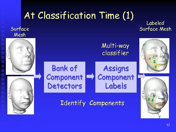At Classification Time (1) Surface Mesh Labeled Surface Mesh Multi-way classifier Bank of Component Detectors Assigns Component Labels Identify Components 32

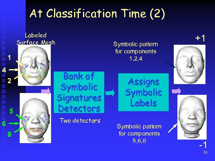At Classification Time (2) Labeled Surface Mesh Symbolic pattern for components 1, 2, 4 1 4 2 5 Bank of Symbolic Signatures Detectors Two detectors 6 8 +1 Assigns Symbolic Labels Symbolic pattern for components 5, 6, 8 -1 33

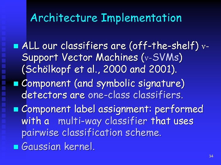Architecture Implementation ALL our classifiers are (off-the-shelf) νSupport Vector Machines (ν-SVMs) (Schölkopf et al. , 2000 and 2001). n Component (and symbolic signature) detectors are one-classifiers. n Component label assignment: performed with a multi-way classifier that uses pairwise classification scheme. n Gaussian kernel. n 34

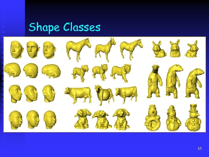Shape Classes 35

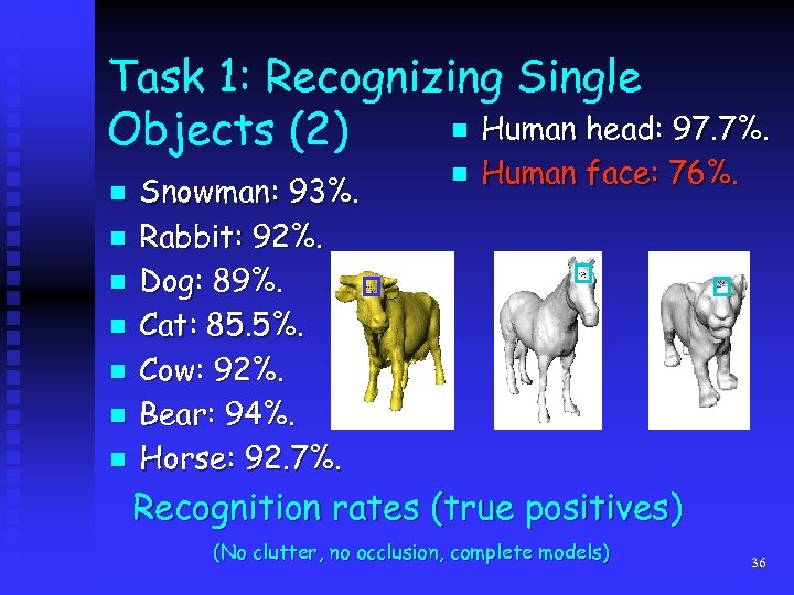Task 1: Recognizing Single n Human head: 97. 7%. Objects (2) n n n n Snowman: 93%. Rabbit: 92%. Dog: 89%. Cat: 85. 5%. Cow: 92%. Bear: 94%. Horse: 92. 7%. n Human face: 76%. Recognition rates (true positives) (No clutter, no occlusion, complete models) 36

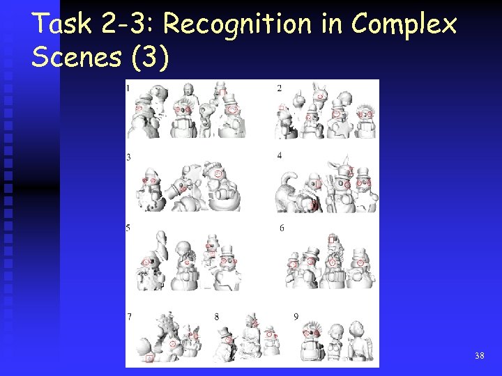
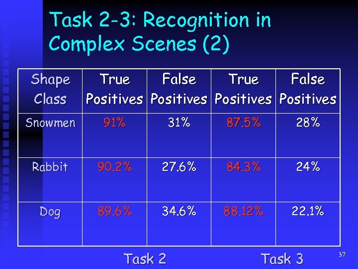Task 2 -3: Recognition in Complex Scenes (2) Shape Class True False Positives Snowmen 91% 31% 87. 5% 28% Rabbit 90. 2% 27. 6% 84. 3% 24% Dog 89. 6% 34. 6% 88. 12% 22. 1% Task 2 Task 3 37

Task 2 -3: Recognition in Complex Scenes (3) 38