Hierarchical Linear Modeling and Related Methods David A

Hierarchical Linear Modeling and Related Methods David A. Hofmann Department of Management Michigan State University Expanded Tutorial SIOP Annual Meeting April 16, 2000 1

Hierarchical Data Structures Ø Hierarchical nature of organizational data – Individuals nested in work groups – Work groups in departments – Departments in organizations – Organizations in environments Ø Consequently, we have constructs that describe: – Individuals – Work groups – Departments – Organizations – Environments 2

Hierarchical Data Structures Ø Hierarchical nature of longitudinal data – Time series nested within individuals – Individuals nested in groups Ø Consequently, we have constructs that describe: – Individuals over time – Individuals – Work groups 3

Click to edit Master title style Theoretical Paradigms Ø Meso Paradigm (House et al. , 1995; Tosi, 1992): – Micro OB – Macro OB – Call for shifting focus: » Contextual variables into Micro theories » Behavioral variables into Macro theories Ø Longitudinal Paradigm (Nesselroade, 1991): – Intraindividual change – Interindividual differences in individual change 4

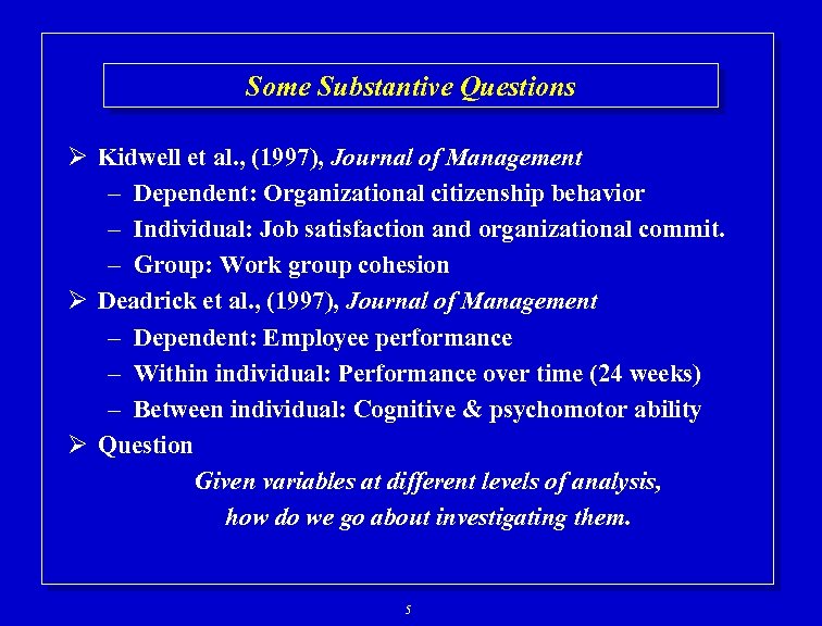Some Substantive Questions Ø Kidwell et al. , (1997), Journal of Management – Dependent: Organizational citizenship behavior – Individual: Job satisfaction and organizational commit. – Group: Work group cohesion Ø Deadrick et al. , (1997), Journal of Management – Dependent: Employee performance – Within individual: Performance over time (24 weeks) – Between individual: Cognitive & psychomotor ability Ø Question Given variables at different levels of analysis, how do we go about investigating them. 5

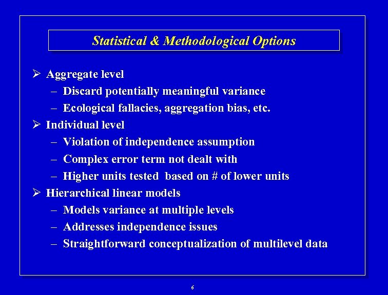Statistical & Methodological Options Ø Aggregate level – Discard potentially meaningful variance – Ecological fallacies, aggregation bias, etc. Ø Individual level – Violation of independence assumption – Complex error term not dealt with – Higher units tested based on # of lower units Ø Hierarchical linear models – Models variance at multiple levels – Addresses independence issues – Straightforward conceptualization of multilevel data 6

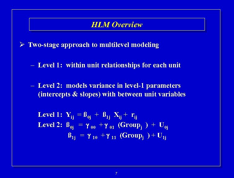HLM Overview Ø Two-stage approach to multilevel modeling – Level 1: within unit relationships for each unit – Level 2: models variance in level-1 parameters (intercepts & slopes) with between unit variables Level 1: Yij = ß 0 j + ß 1 j Xij + rij Level 2: ß 0 j = 00 + 01 (Groupj ) + U 0 j ß 1 j = 10 + 11 (Groupj ) + U 1 j 7

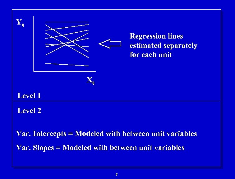Yij Regression lines estimated separately for each unit Xij Level 1 Level 2 Var. Intercepts = Modeled with between unit variables Var. Slopes = Modeled with between unit variables 8

Some Substantive Questions: Applications of HLM Ø Kidwell et al. , (1997), Journal of Management – Individual level job satisfaction and organizational commitment positively related to OCB – Cohesion will be positively related to OCB exhibited by employees beyond that accounted for by satisfaction and commitment – The relationships between commitment/satisfaction and OCB will be stronger in more cohesive groups Ø Deadrick et al. , (1997), Journal of Management – Are there inter-individual differences in performance over time – Do individual differences in ability account for these inter -individual differences 9

HLM Overview Some Preliminary definitions: – Random coefficients/effects » Coefficients/effects that are assumed to vary across units – Common Random coefficients/effects Within unit intercepts Within unit slopes Level 2 residual – Fixed effects » Effects that do not vary across units – Common Fixed effects Level 2 intercept Level 2 slope 10

HLM Overview Ø Estimates provided: – Level 1 parameters (intercepts, slopes) – Level-2 parameters (intercepts, slopes)** – Variance of Level-1 residuals – Variance of Level-2 residuals*** – Covariance of Level-2 residuals Ø Statistical tests: – t-test for parameter estimates (Level-2, fixed effects)** – Chi-Square for variance components (Level-2, random effects)*** 11

A set of example hypotheses: Answering them using HLM 12

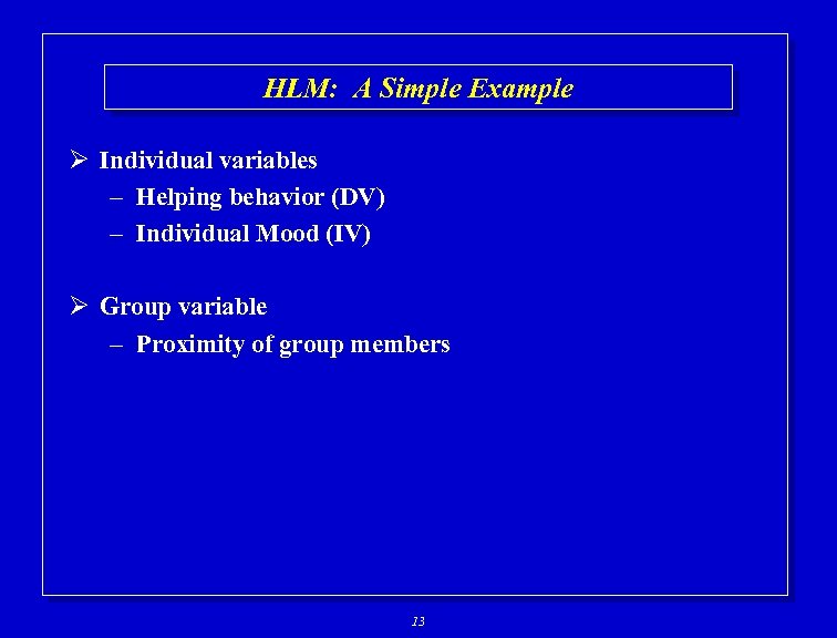HLM: A Simple Example Ø Individual variables – Helping behavior (DV) – Individual Mood (IV) Ø Group variable – Proximity of group members 13

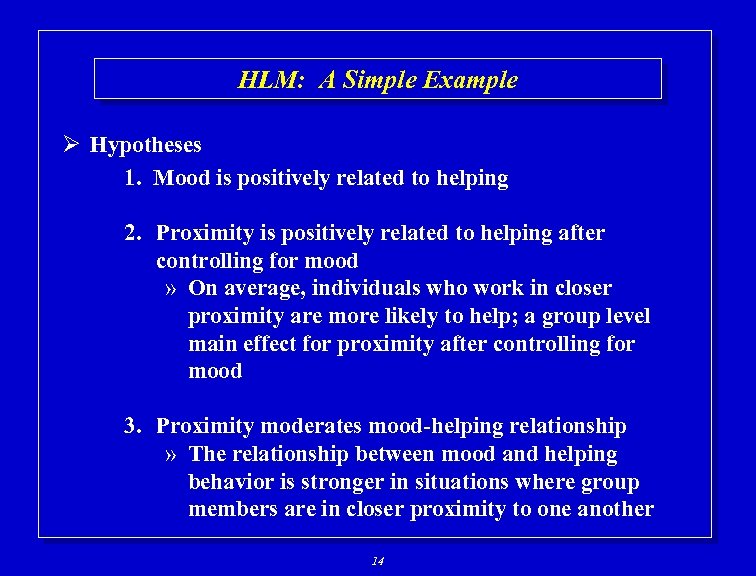HLM: A Simple Example Ø Hypotheses 1. Mood is positively related to helping 2. Proximity is positively related to helping after controlling for mood » On average, individuals who work in closer proximity are more likely to help; a group level main effect for proximity after controlling for mood 3. Proximity moderates mood-helping relationship » The relationship between mood and helping behavior is stronger in situations where group members are in closer proximity to one another 14

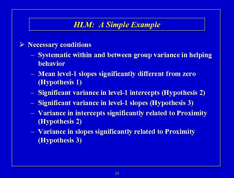HLM: A Simple Example Ø Necessary conditions – Systematic within and between group variance in helping behavior – Mean level-1 slopes significantly different from zero (Hypothesis 1) – Significant variance in level-1 intercepts (Hypothesis 2) – Significant variance in level-1 slopes (Hypothesis 3) – Variance in intercepts significantly related to Proximity (Hypothesis 2) – Variance in slopes significantly related to Proximity (Hypothesis 3) 15

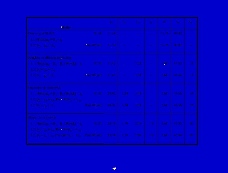
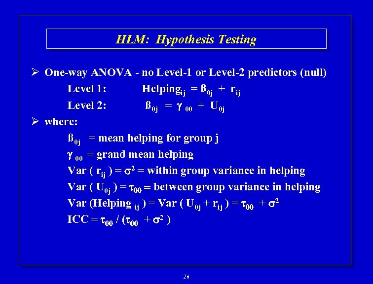HLM: Hypothesis Testing Ø One-way ANOVA - no Level-1 or Level-2 predictors (null) Level 1: Helpingij = ß 0 j + rij Level 2: ß 0 j = 00 + U 0 j Ø where: ß 0 j = mean helping for group j 00 = grand mean helping Var ( rij ) = 2 = within group variance in helping Var ( U 0 j ) = between group variance in helping Var (Helping ij ) = Var ( U 0 j + rij ) = + 2 ICC = / ( + 2 ) 16

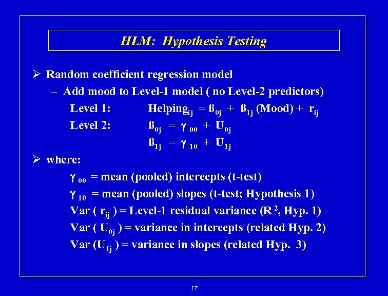HLM: Hypothesis Testing Ø Random coefficient regression model – Add mood to Level-1 model ( no Level-2 predictors) Level 1: Helpingij = ß 0 j + ß 1 j (Mood) + rij Level 2: ß 0 j = 00 + U 0 j ß 1 j = 10 + U 1 j Ø where: 00 = mean (pooled) intercepts (t-test) 10 = mean (pooled) slopes (t-test; Hypothesis 1) Var ( rij ) = Level-1 residual variance (R 2, Hyp. 1) Var ( U 0 j ) = variance in intercepts (related Hyp. 2) Var (U 1 j ) = variance in slopes (related Hyp. 3) 17

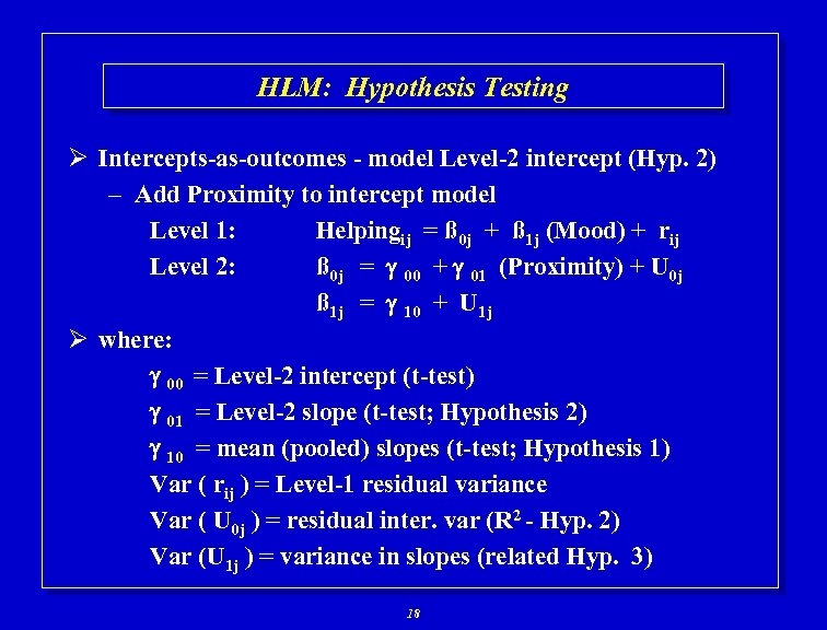HLM: Hypothesis Testing Ø Intercepts-as-outcomes - model Level-2 intercept (Hyp. 2) – Add Proximity to intercept model Level 1: Helpingij = ß 0 j + ß 1 j (Mood) + rij Level 2: ß 0 j = 00 + 01 (Proximity) + U 0 j ß 1 j = 10 + U 1 j Ø where: 00 = Level-2 intercept (t-test) 01 = Level-2 slope (t-test; Hypothesis 2) 10 = mean (pooled) slopes (t-test; Hypothesis 1) Var ( rij ) = Level-1 residual variance Var ( U 0 j ) = residual inter. var (R 2 - Hyp. 2) Var (U 1 j ) = variance in slopes (related Hyp. 3) 18

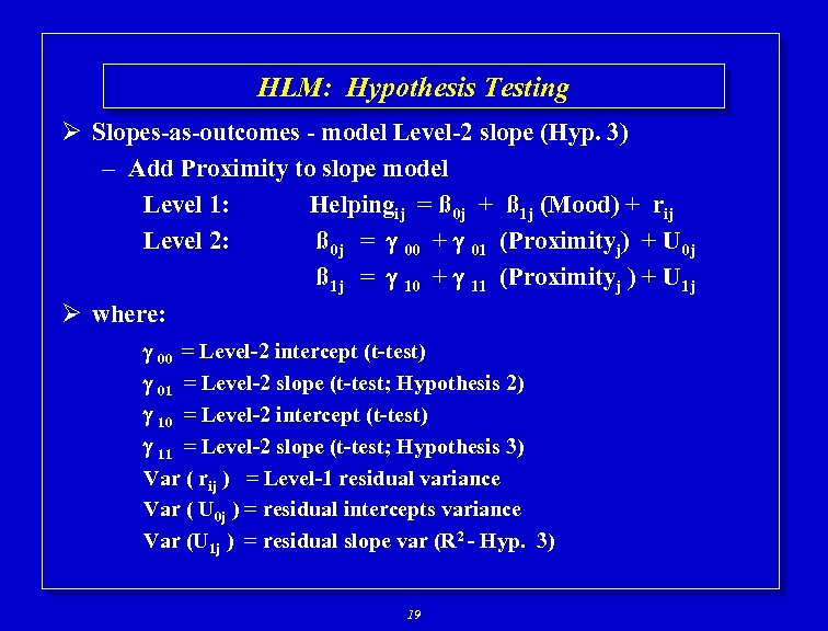HLM: Hypothesis Testing Ø Slopes-as-outcomes - model Level-2 slope (Hyp. 3) – Add Proximity to slope model Level 1: Helpingij = ß 0 j + ß 1 j (Mood) + rij Level 2: ß 0 j = 00 + 01 (Proximityj) + U 0 j ß 1 j = 10 + 11 (Proximityj ) + U 1 j Ø where: 00 = Level-2 intercept (t-test) 01 = Level-2 slope (t-test; Hypothesis 2) 10 = Level-2 intercept (t-test) 11 = Level-2 slope (t-test; Hypothesis 3) Var ( rij ) = Level-1 residual variance Var ( U 0 j ) = residual intercepts variance Var (U 1 j ) = residual slope var (R 2 - Hyp. 3) 19

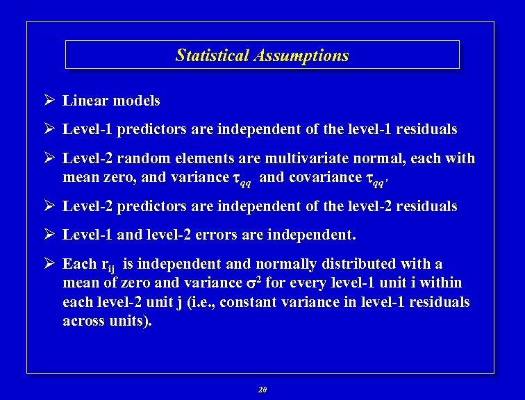Statistical Assumptions Ø Linear models Ø Level-1 predictors are independent of the level-1 residuals Ø Level-2 random elements are multivariate normal, each with mean zero, and variance qq and covariance qq’ Ø Level-2 predictors are independent of the level-2 residuals Ø Level-1 and level-2 errors are independent. Ø Each rij is independent and normally distributed with a mean of zero and variance 2 for every level-1 unit i within each level-2 unit j (i. e. , constant variance in level-1 residuals across units). 20

Statistical Power Ø Kreft (1996) summarized several studies –. 90 power to detect cross-level interactions 30 groups of 30 – Trade-off » Large number of groups, fewer individuals within » Small number of groups, more individuals per group Ø My experience – Cross-level main effects, pretty robust – Cross-level interactions more difficult – Related to within unit standard errors and between group variance 21

Centering Decisions: Scaling of Level-1 Predictors (It’s important and confusing) 22

Centering Decisions Ø Level-1 parameters are used as outcome variables at level-2 Ø Thus, one needs to understand the meaning of these parameters Ø Intercept term: expected value of Y when X is zero Ø Slope term: expected increase in Y for a unit increase in X Ø Raw metric form: X equals zero might not be meaningful 23

Centering Decisions Ø 3 Options – Raw metric – Grand mean – Group mean Ø Kreft et al. (1995): raw metric and grand mean equivalent, group mean non-equivalent Ø Raw metric/Grand mean centering – intercept var = adjusted between group variance in Y Ø Group mean centering – intercept var = between group variance in Y [Kreft, I. G. G. , de Leeuw, J. , & Aiken, L. S. (1995). The effect of different forms of centering in Hierarchical Linear Models. Multivariate Behavioral Research, 30, 1 -21. ] 24

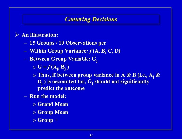Centering Decisions Ø An illustration: – 15 Groups / 10 Observations per – Within Group Variance: f (A, B, C, D) – Between Group Variable: Gj » G = f (Aj, Bj ) » Thus, if between group variance in A & B (i. e. , Aj & Bj ) is accounted for, Gj should not significantly predict the outcome – Run the model: » Grand Mean » Group + 25

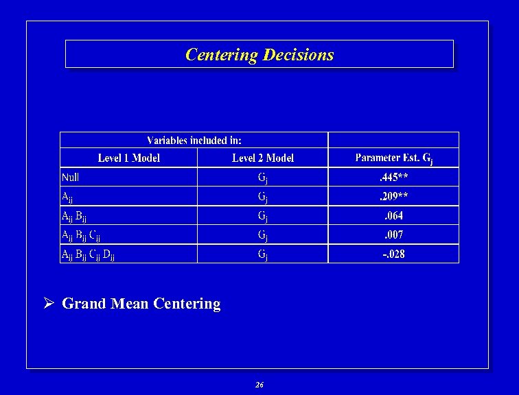Centering Decisions Ø Grand Mean Centering 26

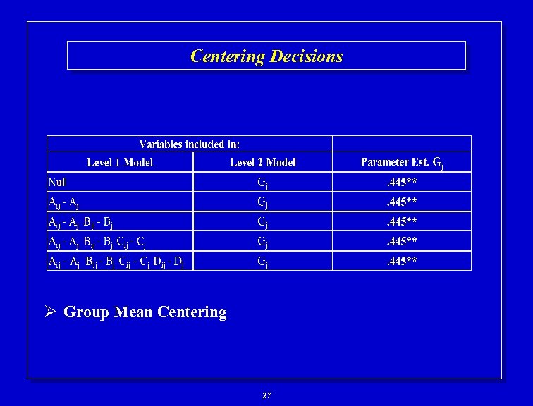Centering Decisions Ø Group Mean Centering 27

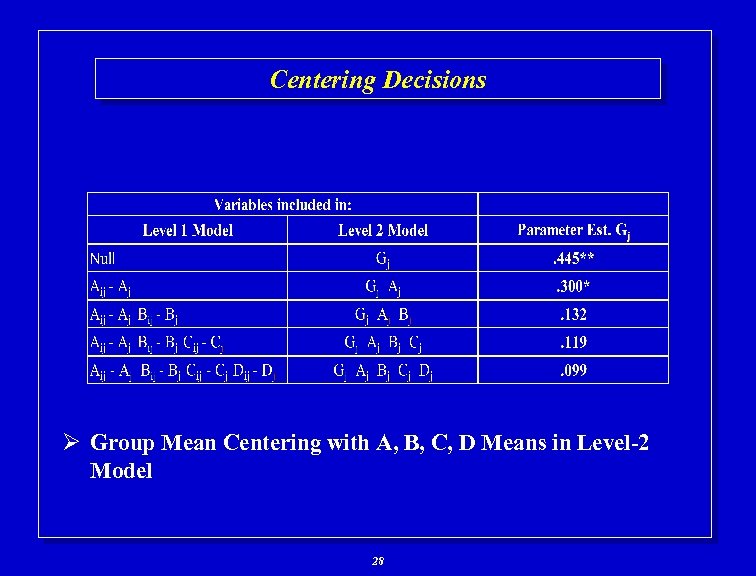Centering Decisions Ø Group Mean Centering with A, B, C, D Means in Level-2 Model 28

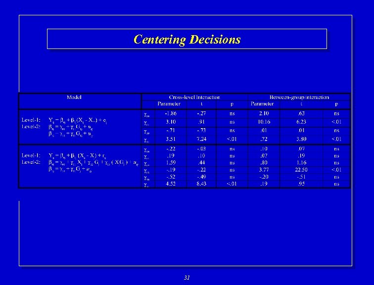
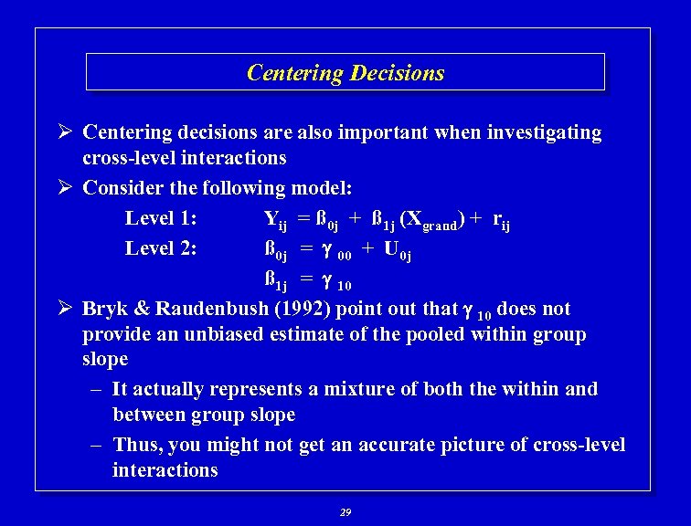Centering Decisions Ø Centering decisions are also important when investigating cross-level interactions Ø Consider the following model: Level 1: Yij = ß 0 j + ß 1 j (Xgrand) + rij Level 2: ß 0 j = 00 + U 0 j ß 1 j = 10 Ø Bryk & Raudenbush (1992) point out that 10 does not provide an unbiased estimate of the pooled within group slope – It actually represents a mixture of both the within and between group slope – Thus, you might not get an accurate picture of cross-level interactions 29

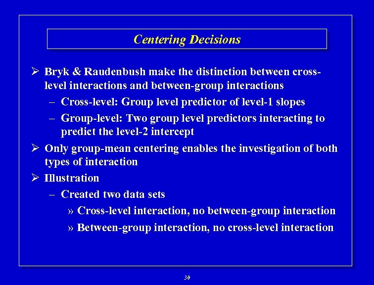Centering Decisions Ø Bryk & Raudenbush make the distinction between crosslevel interactions and between-group interactions – Cross-level: Group level predictor of level-1 slopes – Group-level: Two group level predictors interacting to predict the level-2 intercept Ø Only group-mean centering enables the investigation of both types of interaction Ø Illustration – Created two data sets » Cross-level interaction, no between-group interaction » Between-group interaction, no cross-level interaction 30

Centering Decisions 31

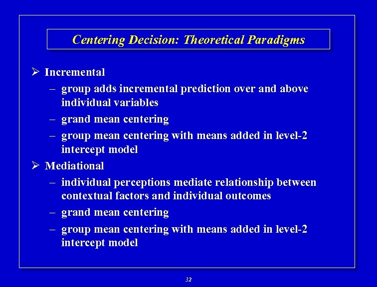Centering Decision: Theoretical Paradigms Ø Incremental – group adds incremental prediction over and above individual variables – grand mean centering – group mean centering with means added in level-2 intercept model Ø Mediational – individual perceptions mediate relationship between contextual factors and individual outcomes – grand mean centering – group mean centering with means added in level-2 intercept model 32

Centering Decisions: Theoretical Paradigms Ø Moderational – group level variable moderates level-1 relationship – group mean centering provides clean estimate of within group slope – separates between group from cross-level interaction – Practical: If running grand mean centered, check final model group mean centered Ø Separate – group mean centering produces separate within and between group structural models 33

Hierarchical Linear Models: Let’s take a look at the software 34

HLM versus OLS regression 35

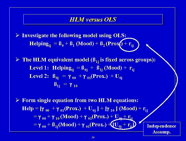HLM versus OLS Ø Investigate the following model using OLS: Helpingij = ß 0 + ß 1 (Mood) + ß 2 (Prox. ) + rij Ø The HLM equivalent model (ß 1 j is fixed across groups): Level 1: Helpingij = ß 0 j + ß 1 j (Mood) + rij Level 2: ß 0 j = 00 + 01(Prox. ) + U 0 j ß 1 j = 10 Ø Form single equation from two HLM equations: Help = [ 00 + 01(Prox. ) + U 0 j ] + [ 10 ] (Mood) + rij = 00 + 10 (Mood) + 01(Prox. ) + U 0 j + rij = 00 + ß 1 j(Mood) + 01(Prox. ) + [U 0 j + rij] Independence Assump. 36

HLM Estimation: A brief overview 37

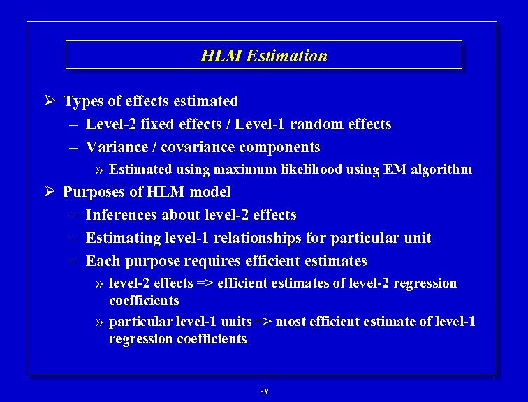HLM Estimation Ø Types of effects estimated – Level-2 fixed effects / Level-1 random effects – Variance / covariance components » Estimated using maximum likelihood using EM algorithm Ø Purposes of HLM model – Inferences about level-2 effects – Estimating level-1 relationships for particular unit – Each purpose requires efficient estimates » level-2 effects => efficient estimates of level-2 regression coefficients » particular level-1 units => most efficient estimate of level-1 regression coefficients 38

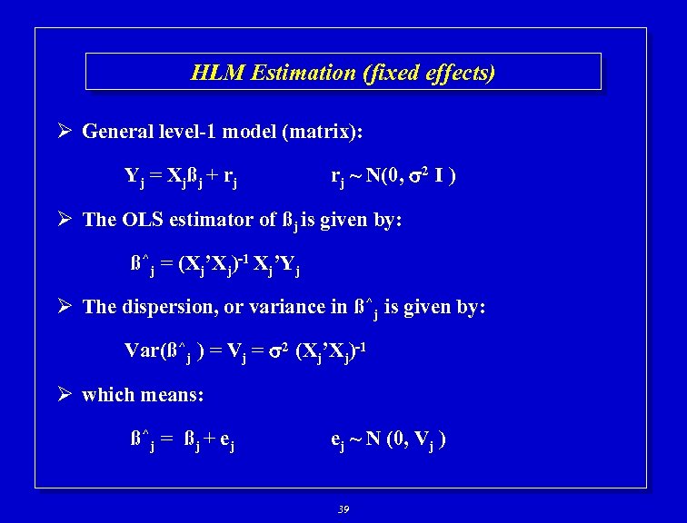HLM Estimation (fixed effects) Ø General level-1 model (matrix): Y j = X jß j + r j rj ~ N(0, 2 I ) Ø The OLS estimator of ßj is given by: ß^j = (Xj’Xj)-1 Xj’Yj Ø The dispersion, or variance in ß^j is given by: Var(ß^j ) = Vj = 2 (Xj’Xj)-1 Ø which means: ß ^j = ß j + e j ej ~ N (0, Vj ) 39

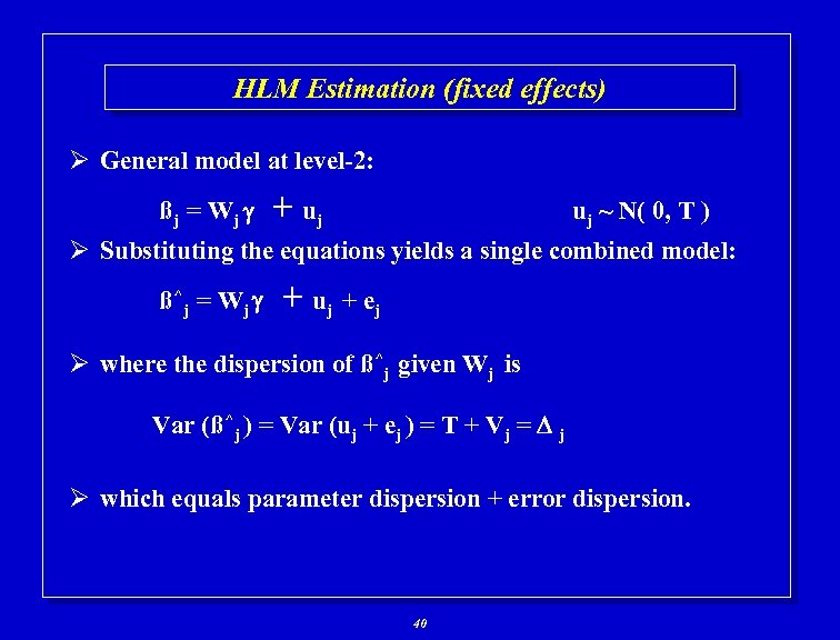HLM Estimation (fixed effects) Ø General model at level-2: ßj = W j + uj uj ~ N( 0, T ) Ø Substituting the equations yields a single combined model: ß ^j = W j + uj + e j Ø where the dispersion of ß^j given Wj is Var (ß^j ) = Var (uj + ej ) = T + Vj = j Ø which equals parameter dispersion + error dispersion. 40

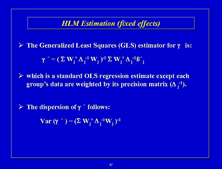HLM Estimation (fixed effects) Ø The Generalized Least Squares (GLS) estimator for is: ^ = ( Wj’ j-1 Wj )-1 Wj’ j-1ß^j Ø which is a standard OLS regression estimate except each group’s data are weighted by its precision matrix ( j-1). Ø The dispersion of ^ follows: Var ( ^ ) = ( Wj’ j-1 Wj )-1 41

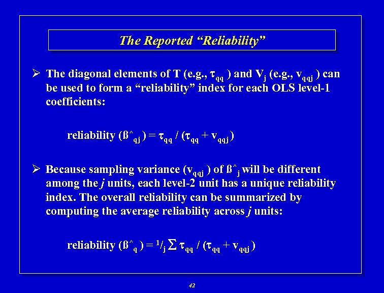The Reported “Reliability” Ø The diagonal elements of T (e. g. , qq ) and Vj (e. g. , vqqj ) can be used to form a “reliability” index for each OLS level-1 coefficients: reliability (ß^qj ) = qq / ( qq + vqqj ) Ø Because sampling variance (vqqj ) of ß^j will be different among the j units, each level-2 unit has a unique reliability index. The overall reliability can be summarized by computing the average reliability across j units: reliability (ß^q ) = 1/j qq / ( qq + vqqj ) 42

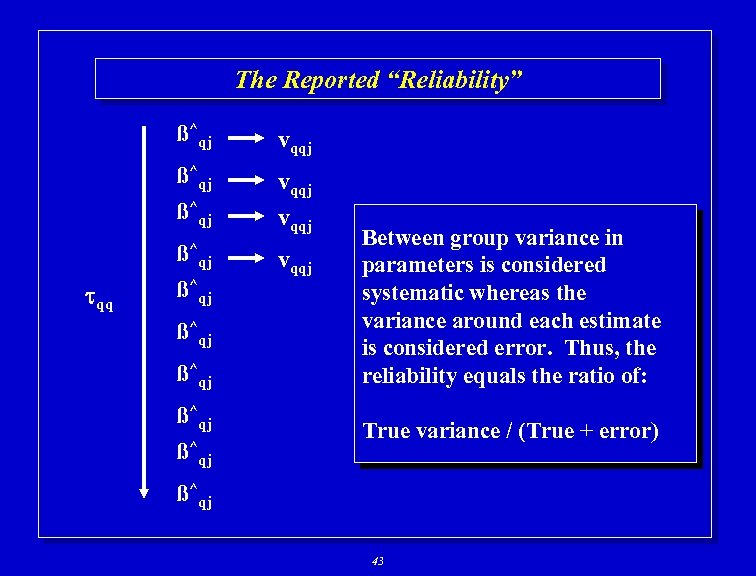The Reported “Reliability” ß^qj vqqj ß^ qq vqqj qj ß^qj ß^qj Between group variance in parameters is considered systematic whereas the variance around each estimate is considered error. Thus, the reliability equals the ratio of: True variance / (True + error) ß^qj 43

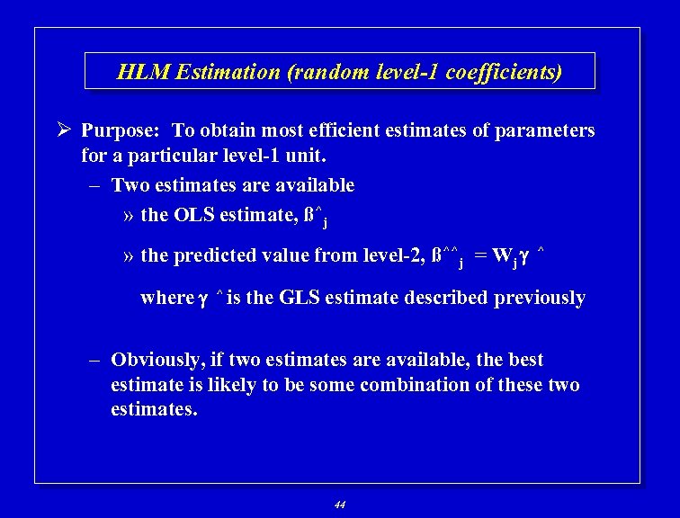HLM Estimation (random level-1 coefficients) Ø Purpose: To obtain most efficient estimates of parameters for a particular level-1 unit. – Two estimates are available » the OLS estimate, ß^j » the predicted value from level-2, ß^^j = Wj ^ where ^ is the GLS estimate described previously – Obviously, if two estimates are available, the best estimate is likely to be some combination of these two estimates. 44

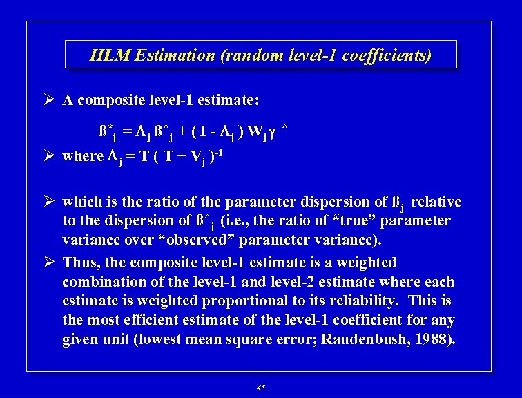HLM Estimation (random level-1 coefficients) Ø A composite level-1 estimate: ß*j = j ß^j + ( I - j ) Wj ^ Ø where j = T ( T + Vj )-1 Ø which is the ratio of the parameter dispersion of ßj relative to the dispersion of ß^j (i. e. , the ratio of “true” parameter variance over “observed” parameter variance). Ø Thus, the composite level-1 estimate is a weighted combination of the level-1 and level-2 estimate where each estimate is weighted proportional to its reliability. This is the most efficient estimate of the level-1 coefficient for any given unit (lowest mean square error; Raudenbush, 1988). 45

Do You Really Need HLM? Alternatives for Estimating Hierarchical Models Part I: Cross Level Models 46

SAS: Proc Mixed Ø SAS Proc Mixed will estimate these models Ø Key components of Proc Mixed command language – Proc mixed » Class – Group identifier » Model – Regression equation including both individual, group, and interactions (if applicable) » Random – Specification of random effects (those allowed to vary across groups) 47

SAS: Proc Mixed Ø Key components of Proc Mixed command language – Some options you might want to select » Class: noitprint (suppresses interation history) » Model: – solution (prints solution for random effects) – ddfm=bw (specifies the “between/within” method for computing denominator degrees of freedom for tests of fixed effects) » Random: – sub= id (how level-1 units are divided into level-2 units) – type=un (specifies unstructured variance-covariance matrix of intercepts and slopes; i. e. , allows parameters to be determined by data) 48

SAS: Proc Mixed 49

SAS: Proc Mixed Ø Key references – Singer, J. (1998). Using SAS PROC MIXED to fit multilevel models, hierarchical models, and individual growth models. Journal of Educational and Behavioral Statistics, 23, 323 -355. Ø Available on her homepage – http: //hugse 1. harvard. edu/~faculty/singer/ 50

Do You Really Need HLM? Alternatives for Estimating Hierarchical Models Part II: Longitudinal Models 51

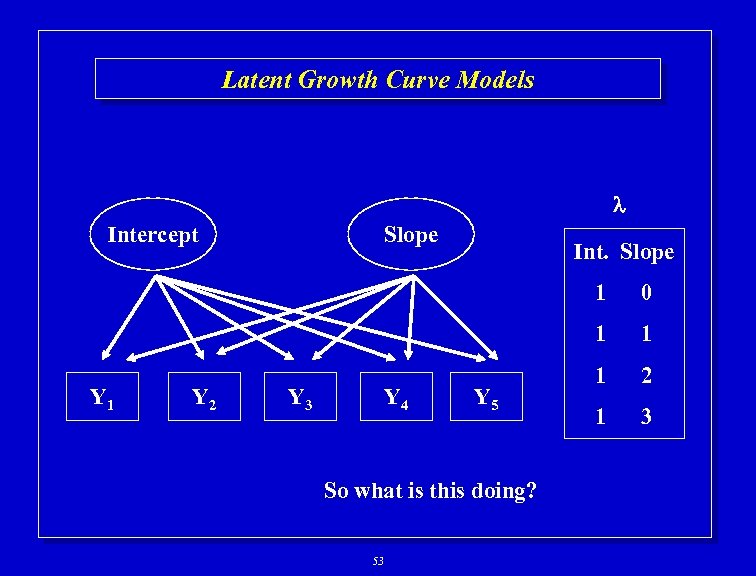
Latent Growth Curve Models Ø Structural equation programs can be used to model – Interindividual differences in intraindividual change – Predictors of these change patterns Ø How does it work – Analyze covariance matrix of interrelationships among repeated measures of outcome – “Flip” the logic of factor analysis » Typically program estimates factor loadings and factors are interpreted in relation to factor loadings » In these models, you fix all of the factor loadings and interpret variance in factors in accordance to factor loadings that you specify 52

Latent Growth Curve Models Intercept Slope Int. Slope 1 1 Y 2 Y 3 Y 4 Y 5 So what is this doing? 53 0 1 1 2 1 3

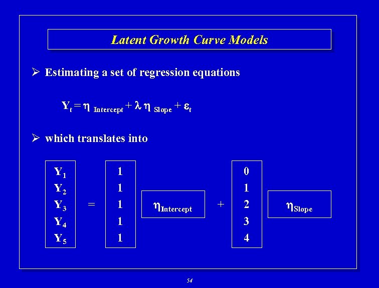Latent Growth Curve Models Ø Estimating a set of regression equations Yt = Intercept + Slope + t Ø which translates into Y 1 Y 2 Y 3 Y 4 Y 5 = 1 1 1 Intercept 54 + 0 1 2 3 4 Slope

Latent Growth Curve Models Ø Variance in factors – Individual differences in intercepts and slopes – Why » In factors analysis, variance in factors equals variability across persons on latent construct » Could create a factor score for each individual; variability in factor scores conceptually represents variance in factor across persons » Same applies here – Fixing factor loadings defines factors as intercept and linear trend – Variance in factors represents variance across persons in intercepts and slopes 55

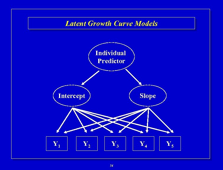Latent Growth Curve Models Individual Predictor Intercept Y 1 Y 2 Slope Y 3 56 Y 4 Y 5

Latent Growth Curve Models Ø Key references – Mc. Ardle, J. J. , & Epstein, D. (1987). Latent growth curves within developmental structural equation models. Child Development, 58, 110 -133. – Muthen, B. O. (1991). Analysis of longitudinal data using latent variable models with varying parameters. In L. M. Collins, & J. L. Horn, (Eds. ), Best Methods for the Analysis of Change (pp. 37 -54). – Ployhart, R. E. , & Hakel, M. D. (1998). The substantive nature of performance variability: Predicting interindividual differences in intraindividual change. Personnel Psychology, 51, 859 -901. – Chan, D. (1998). The conceptualization and analysis of change over time: An integrative approach to incorporating longitudinal mean and covariance structures analysis (LMACS) and multiple indicator latent growth modeling (MLGM). Organizational Research Methods, 1, 421 -483. 57

Questions: About Today or About Your Own Research 58