Hedonic Imputed Housing Price Indices from a Model

Hedonic Imputed Housing Price Indices from a Model with Dynamic Shadow Prices Incorporating Nearest Neighbour Information Harry T. Cominos University of Queensland Supervisors: Prasada Rao; Alicia Rambaldi

Structure of Presentation 1. 2. 3. 4. 5. 6. Background and Motivation Existing Hedonic Methods for House Price Indexes Hedonic Specification with Spatial Autocorrelation. Hedonic Specification with Dynamic coefficients Data (Brisbane Metropolitan Area) Empirical Results

Background & Motivation n 1. 2. n 2 main issues in house price index construction: Quality change problem Compositional change problem. The hedonic method (theoretically) accounts for both quality and compositional changes over time.

Hedonic Method n Regression based – Explains the price of a house using a range of characteristics. n Drawback – Data Intensive. n The hedonic approach has led to the 1. Time-dummy variable method (DTH) Hedonic Imputation method (HI) Characteristics Price Method (CP). 2. 3.

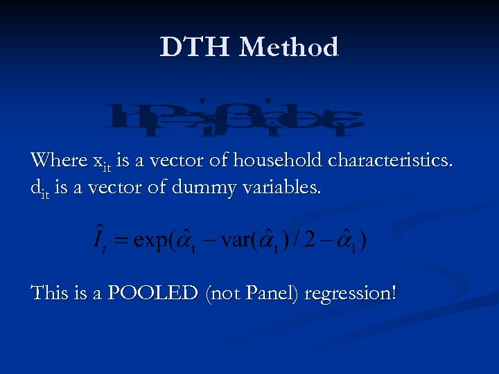DTH Method Where xit is a vector of household characteristics. dit is a vector of dummy variables. This is a POOLED (not Panel) regression!

DTH Method n DTH Method assumes same hedonic model and characteristics in every period. n It is less restrictive to use the adjacentperiod approach (AP-DTH). Ie. regression is estimated for every pair of periods. n There is no choice of index number formula for DTH and AP-DTH.

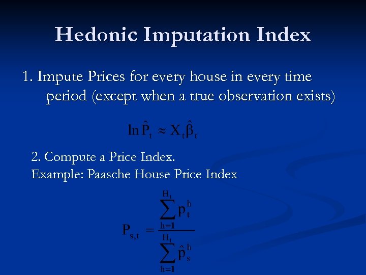
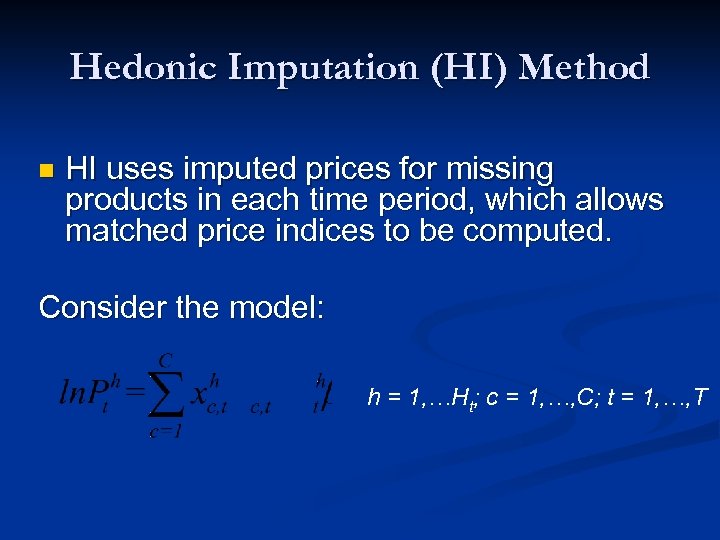Hedonic Imputation (HI) Method n HI uses imputed prices for missing products in each time period, which allows matched price indices to be computed. Consider the model: h = 1, …Ht; c = 1, …, C; t = 1, …, T

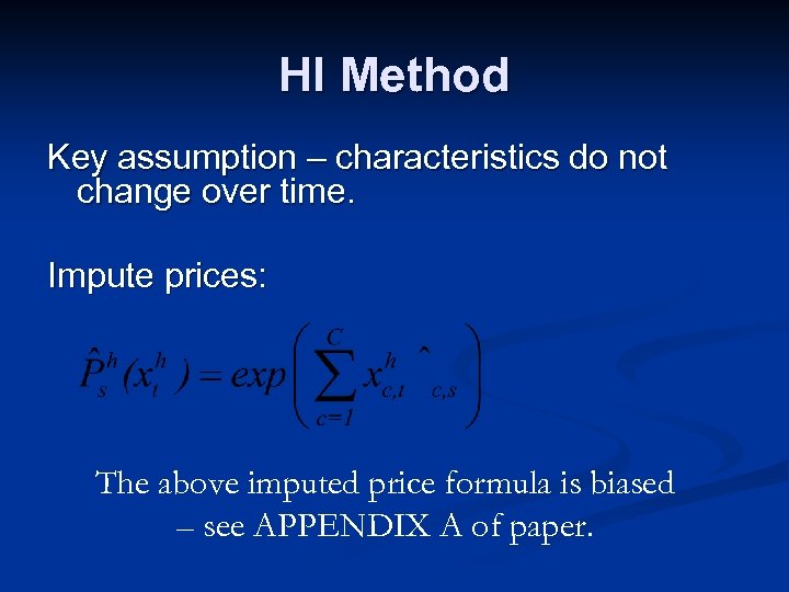HI Method Key assumption – characteristics do not change over time. Impute prices: The above imputed price formula is biased – see APPENDIX A of paper.

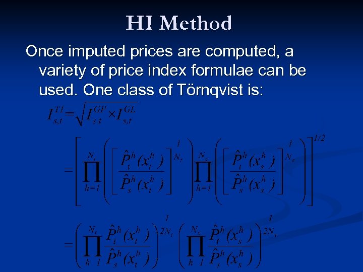HI Method Once imputed prices are computed, a variety of price index formulae can be used. One class of Törnqvist is:

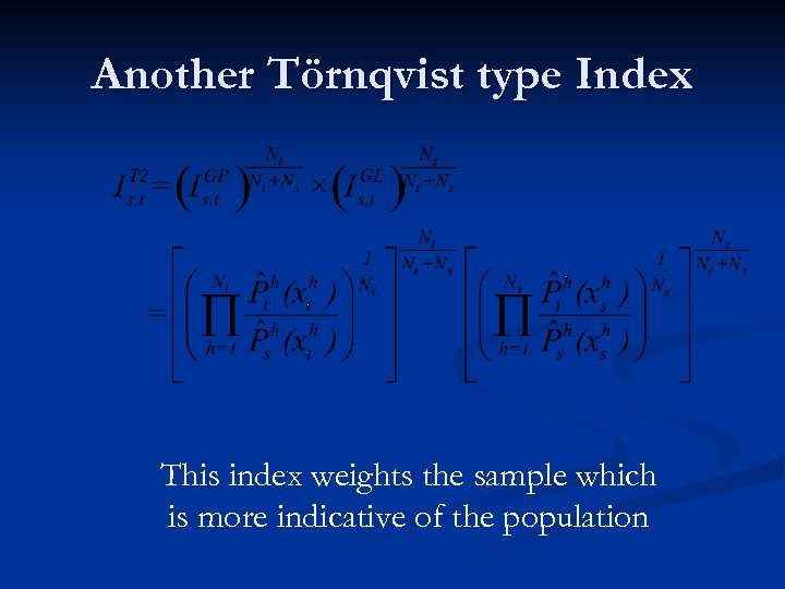Another Törnqvist type Index This index weights the sample which is more indicative of the population

Hedonic Specification with Spatial Autocorrelation House prices should be spatially autocorrelated because neighbourhoods 1. Have similar structural characteristics (block size, age) 2. Share location amenities (supermarkets, schools) 3. Share socioeconomic variables (local crime rates, wealth levels)

Hedonic Specification with Spatial Autocorrelation Most empirical examples of Hedonic Indexes assume white noise errors, but… In practice, the residuals should be spatially autocorrelated because the hedonic function is not fully specified (due to data constraints).

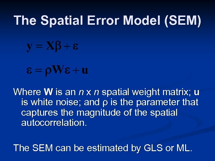The Spatial Error Model (SEM) Where W is an n x n spatial weight matrix; u is white noise; and ρ is the parameter that captures the magnitude of the spatial autocorrelation. The SEM can be estimated by GLS or ML.

Spatial weight matrix (W) W has elements representing the spatial relationship between houses i and j. The researcher take the specification of W as known a priori. Common properties: n W is non-negative n wii = 0 (ie. an observation does not affect its own prediction)

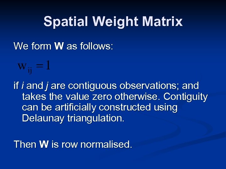Spatial Weight Matrix We form W as follows: if i and j are contiguous observations; and takes the value zero otherwise. Contiguity can be artificially constructed using Delaunay triangulation. Then W is row normalised.

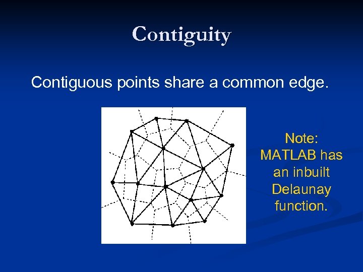Contiguity Contiguous points share a common edge. Note: MATLAB has an inbuilt Delaunay function.

Spatial Weight Matrix In order to construct W in this manner, the latitude and longitude coordinate of each house must be known. This allows R. Kelley Pace’s FDELW 2 Matlab function to be used to convert the Delaunay algorithm results into a contiguity matrix.

Hedonic Specification with Dynamic coefficients So far hedonic parameters have been • constrained to be constant over the sample period of interest (ie. the DTH method) or • allowed to vary in a sporadic fashion because the hedonic regression is reestimated in every time period (or every second period for AP-DTH).

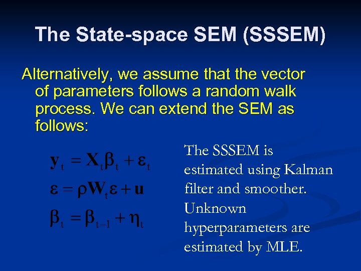The State-space SEM (SSSEM) Alternatively, we assume that the vector of parameters follows a random walk process. We can extend the SEM as follows: The SSSEM is estimated using Kalman filter and smoother. Unknown hyperparameters are estimated by MLE.

Data n n n 1. 2. 3. Data compiled from property information service RP DATA, from www. rpdata. com Website is search engine based. Data preparation: Raw data downloaded and hedonics chosen. Data were filtered. Address of each house was geocoded to provide lat/long

Data n n n Initially 316, 359 observations from early 50 s to 12/05. Most observations did not contain info on property attributes. Of those observations containing hedonics, reporting was inconsistent. Hence, only ADDRESS, PRICE, DATE, AREA, BED, BATH, CARLUG information was kept. After filtering, 71, 583 remaining observations spanning 01/71 – 12/05

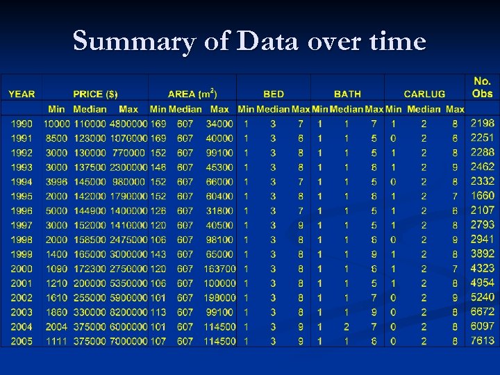Summary of Data over time

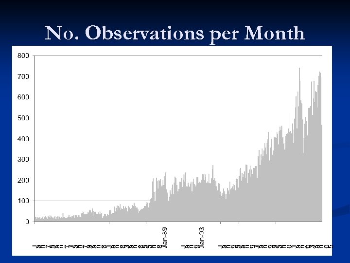No. Observations per Month

Data Limitations Data could not be downloaded for all suburbs. n With an extensive list of property attributes, it would be great to use some of this information! (POOL etc) n Tedious and time consuming to compile data. n

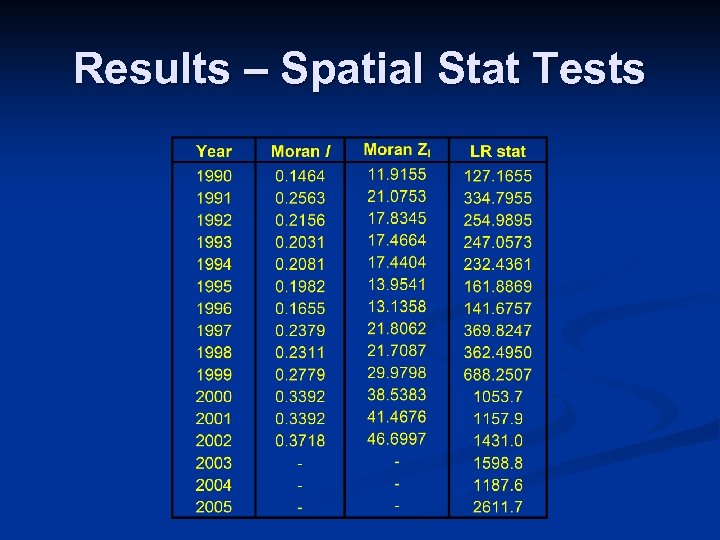Results – Spatial Stat Tests

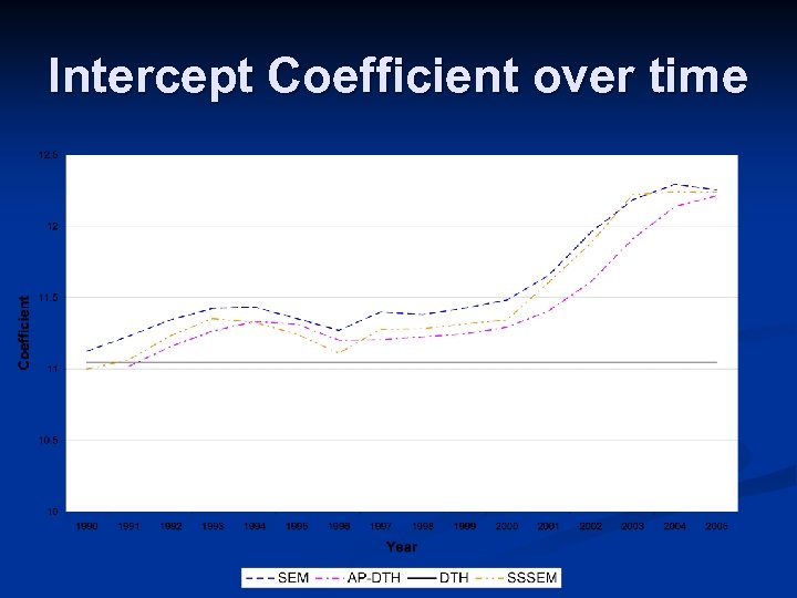Intercept Coefficient over time

AREA coefficient over time

BED coefficient over time

BATH coefficient over time

Shadow Prices for AP-DTH

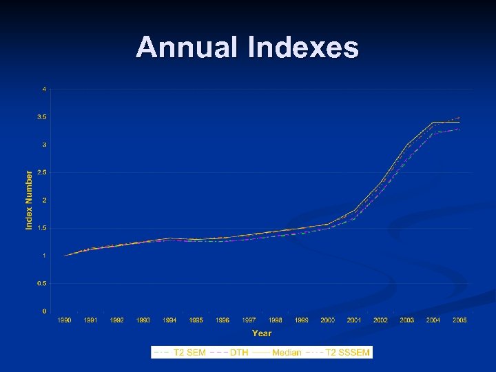Annual Indexes

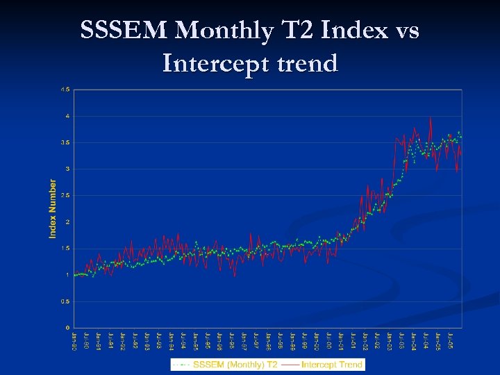SSSEM Monthly T 2 Index vs Intercept trend

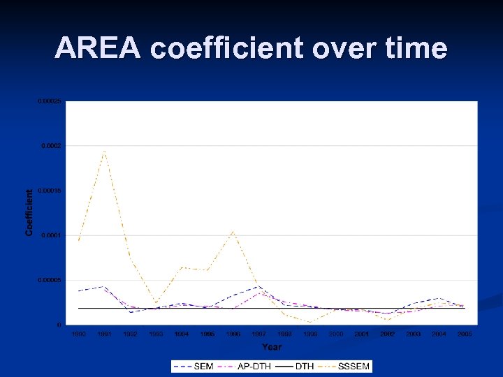
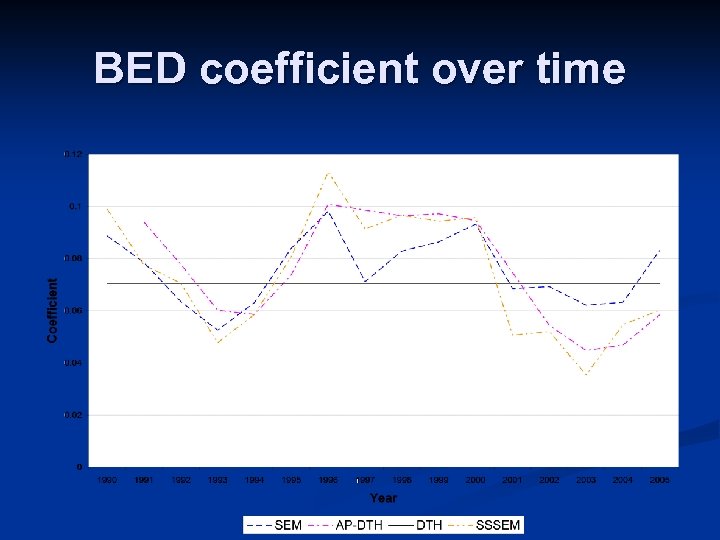
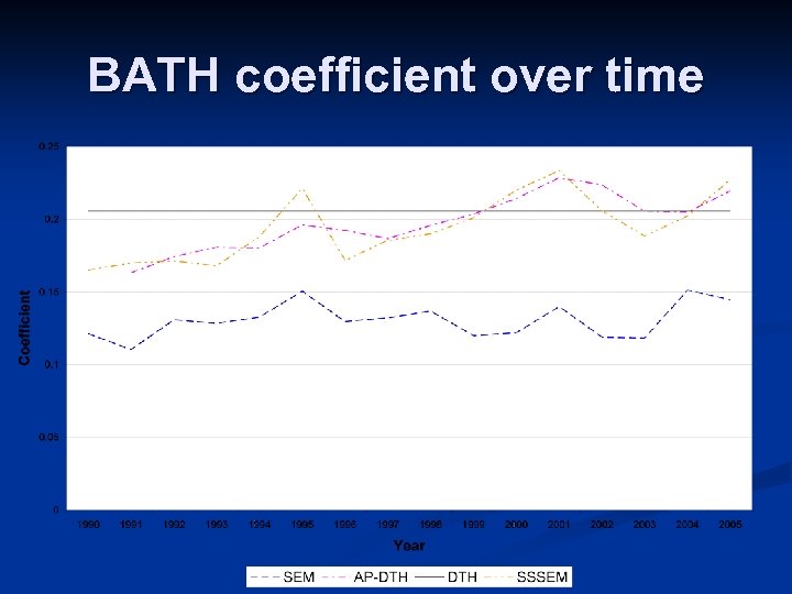
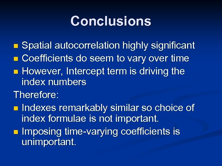Conclusions Spatial autocorrelation highly significant n Coefficients do seem to vary over time n However, Intercept term is driving the index numbers Therefore: n Indexes remarkably similar so choice of index formulae is not important. n Imposing time-varying coefficients is unimportant. n

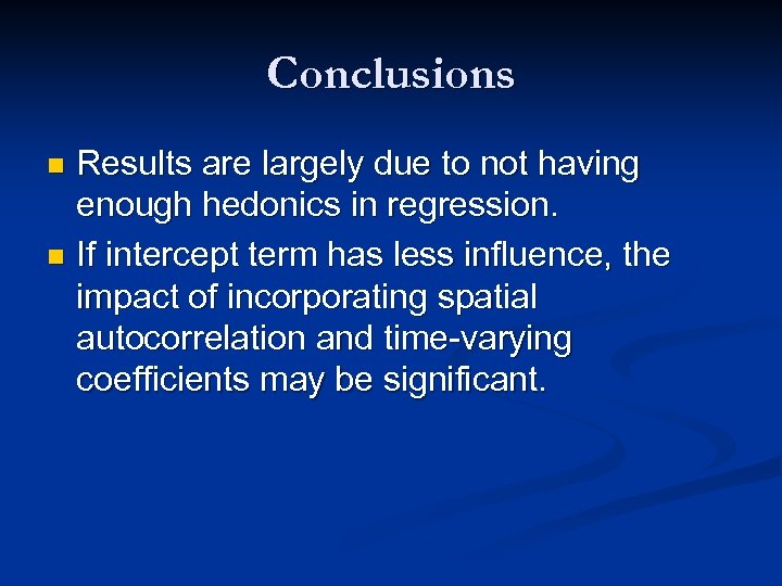Conclusions Results are largely due to not having enough hedonics in regression. n If intercept term has less influence, the impact of incorporating spatial autocorrelation and time-varying coefficients may be significant. n

Future research Different Weight matrices in lattice models. n Geostatistical models n HI and CP indexes particular to housing case. n Robust method to adjust for unusual observations such as acreage properties n Adjust/test for seasonality n DATA DATA n

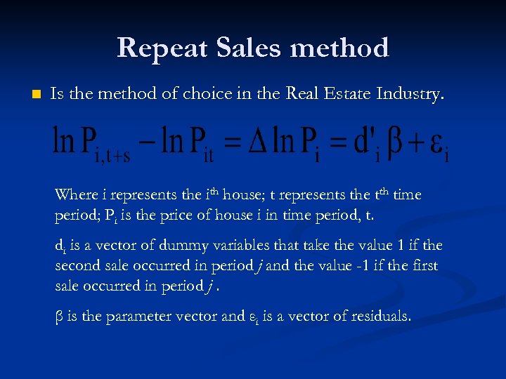Repeat Sales method n Is the method of choice in the Real Estate Industry. Where i represents the ith house; t represents the tth time period; Pi is the price of house i in time period, t. di is a vector of dummy variables that take the value 1 if the second sale occurred in period j and the value -1 if the first sale occurred in period j. β is the parameter vector and εi is a vector of residuals.

Repeat Sales Method Weaknesses: 1. It does not make maximum use of the available data. 2. It violates temporal fixity. 3. Does not account for the depreciation effect. 4. Repeat sales properties may differ in some respects from single sale properties.

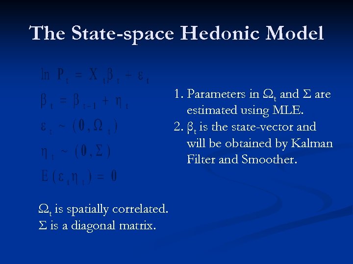The State-space Hedonic Model 1. Parameters in Ωt and Σ are estimated using MLE. 2. βt is the state-vector and will be obtained by Kalman Filter and Smoother. Ωt is spatially correlated. Σ is a diagonal matrix.

Hedonic Imputation Index 1. Impute Prices for every house in every time period (except when a true observation exists) 2. Compute a Price Index. Example: Paasche House Price Index

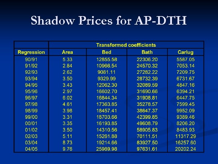
Summary Using a State-Space Formulation of a Hedonic Model, and a Hedonic Imputation Index has the following advantages: n The shadow prices of characteristics vary over time. n Spatial correlation is accounted for in the estimation process. n The resulting Index satisfies temporal fixity.

Summary Makes maximum use of the available data. n Takes into account shifts in the composition of transactions each period. n Controls for quality Improvements (Data dependent) n

Incorporating Spatial Correlation 1. 2. 3. 4. Collect House Price Data for Brisbane – which includes the address of each house. Change addresses to Latitudes/longitudes Use the Lat/Long to calculate distance between a house and its ‘nearest neighbours’. Use this information in the Model.