dfacb8289ba7429c2eaf3d0fb7280b5a.ppt
- Количество слайдов: 51
Haskins f. MRI Workshop Part II: Single Subject Analysis - Event & Block Designs
Analysis Strategy Overview 1) “massively univariate” approach 2) two-stage analysis: a) single-subject regression on time-course data b) across-subject t-test on subject effects c) why? simpler. . .
Block & Event-Related Designs Block designs 1) task or condition alternates at ~20 second intervals 2) analysis looks for differences in the mean response level across the entire block 3) Event-related designs 4) random order of stimulus types 5) analysis extracts the simple “evoked” response to each stimulus type; then assesses differences among types
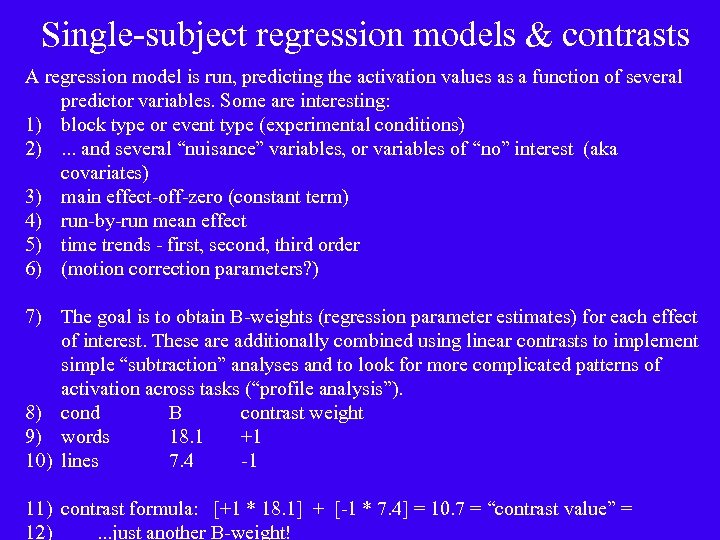
Single-subject regression models & contrasts A regression model is run, predicting the activation values as a function of several predictor variables. Some are interesting: 1) block type or event type (experimental conditions) 2). . . and several “nuisance” variables, or variables of “no” interest (aka covariates) 3) main effect-off-zero (constant term) 4) run-by-run mean effect 5) time trends - first, second, third order 6) (motion correction parameters? ) 7) The goal is to obtain B-weights (regression parameter estimates) for each effect of interest. These are additionally combined using linear contrasts to implement simple “subtraction” analyses and to look for more complicated patterns of activation across tasks (“profile analysis”). 8) cond B contrast weight 9) words 18. 1 +1 10) lines 7. 4 -1 11) contrast formula: [+1 * 18. 1] + [-1 * 7. 4] = 10. 7 = “contrast value” = 12). . . just another B-weight!
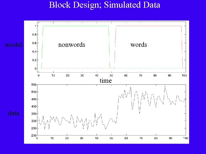
Block Design; Simulated Data model nonwords time data
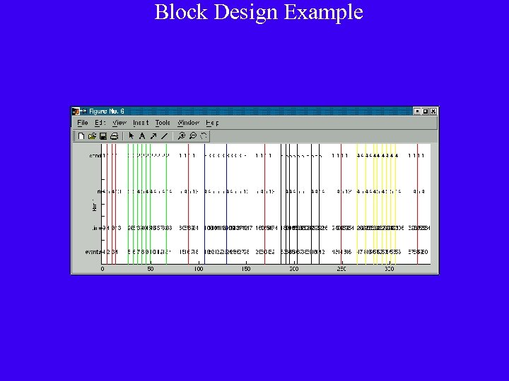
Block Design Example
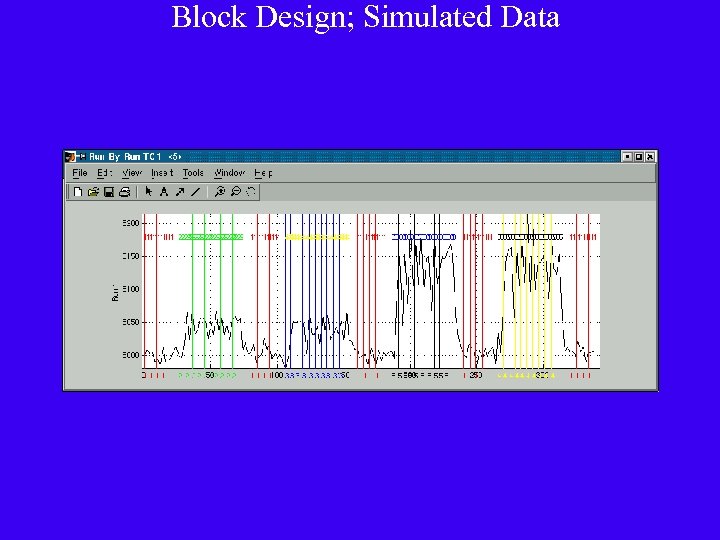
Block Design; Simulated Data
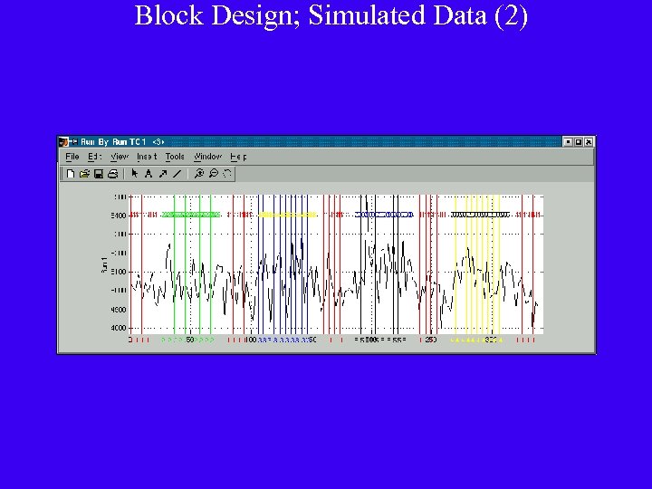
Block Design; Simulated Data (2)
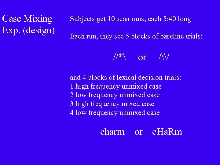
Case Mixing Exp. (design) Subjects get 10 scan runs, each 5: 40 long Each run, they see 5 blocks of baseline trials: //* or /\/ and 4 blocks of lexical decision trials: 1 high frequency unmixed case 2 low frequency unmixed case 3 high frequency mixed case 4 low frequency unmixed case charm or c. Ha. Rm
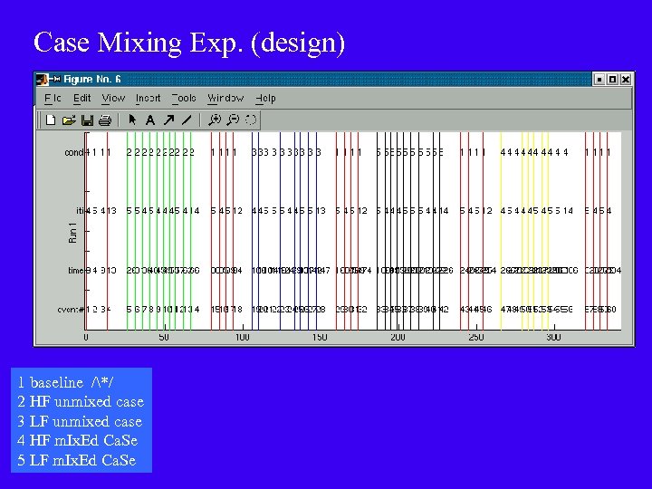
Case Mixing Exp. (design) 1 baseline /*/ 2 HF unmixed case 3 LF unmixed case 4 HF m. Ix. Ed Ca. Se 5 LF m. Ix. Ed Ca. Se
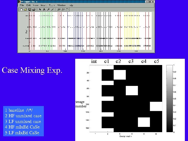
int Case Mixing Exp. 1 baseline /*/ 2 HF unmixed case 3 LF unmixed case 4 HF m. Ix. Ed Ca. Se 5 LF m. Ix. Ed Ca. Se image number c 1 c 2 c 3 c 4 c 5
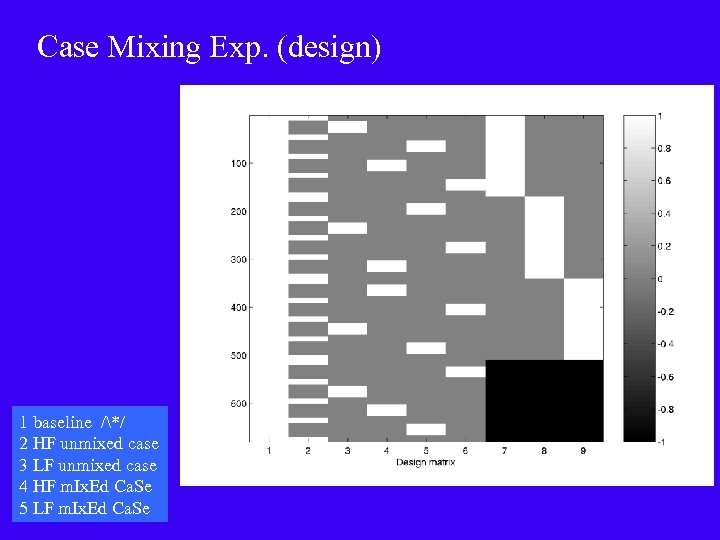
Case Mixing Exp. (design) 1 baseline /*/ 2 HF unmixed case 3 LF unmixed case 4 HF m. Ix. Ed Ca. Se 5 LF m. Ix. Ed Ca. Se
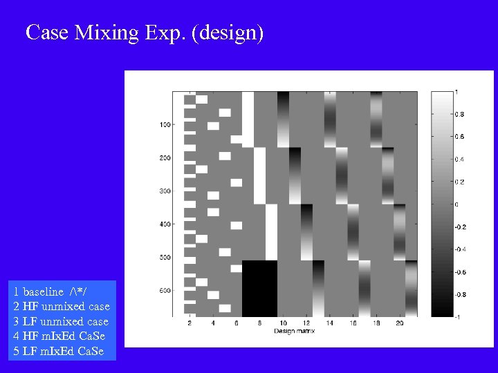
Case Mixing Exp. (design) 1 baseline /*/ 2 HF unmixed case 3 LF unmixed case 4 HF m. Ix. Ed Ca. Se 5 LF m. Ix. Ed Ca. Se
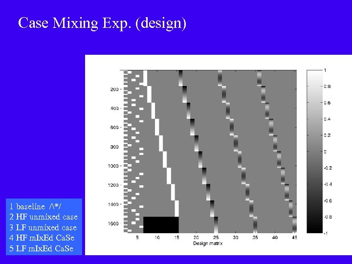
Case Mixing Exp. (design) 1 baseline /*/ 2 HF unmixed case 3 LF unmixed case 4 HF m. Ix. Ed Ca. Se 5 LF m. Ix. Ed Ca. Se
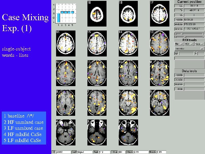
Case Mixing Exp. (1) single-subject words - lines 1 baseline /*/ 2 HF unmixed case 3 LF unmixed case 4 HF m. Ix. Ed Ca. Se 5 LF m. Ix. Ed Ca. Se
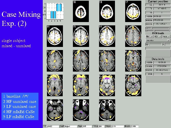
Case Mixing Exp. (2) single subject mixed - unmixed 1 baseline /*/ 2 HF unmixed case 3 LF unmixed case 4 HF m. Ix. Ed Ca. Se 5 LF m. Ix. Ed Ca. Se
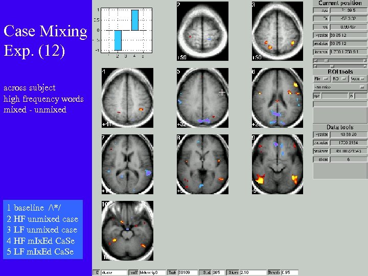
Case Mixing Exp. (12) across subject high frequency words mixed - unmixed 1 baseline /*/ 2 HF unmixed case 3 LF unmixed case 4 HF m. Ix. Ed Ca. Se 5 LF m. Ix. Ed Ca. Se
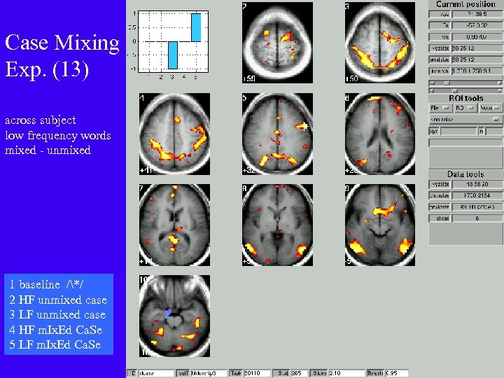
Case Mixing Exp. (13) across subject low frequency words mixed - unmixed 1 baseline /*/ 2 HF unmixed case 3 LF unmixed case 4 HF m. Ix. Ed Ca. Se 5 LF m. Ix. Ed Ca. Se
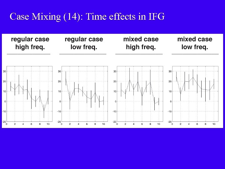
Case Mixing (14): Time effects in IFG
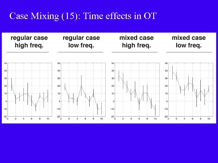
Case Mixing (15): Time effects in OT
Event-Related Designs, Two Analyses 1) Using a priori predicted response functions a) long intertrial interval designs b) Reference waveform regression 2) Estimating the actual response a) simple averaging b) delta function regression (FIR, finite impulse response) 3) Some examples
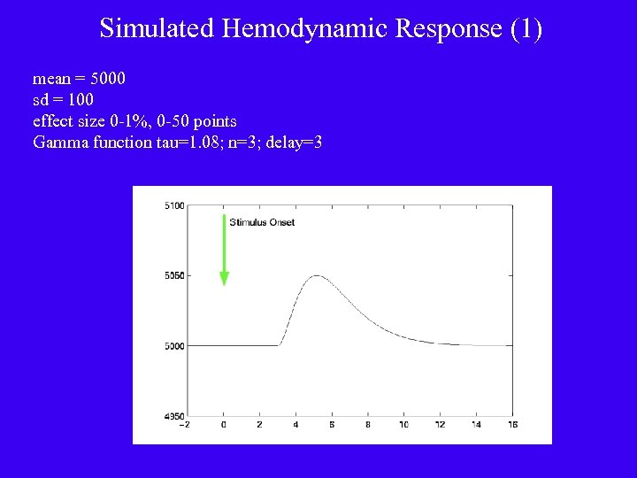
Simulated Hemodynamic Response (1) mean = 5000 sd = 100 effect size 0 -1%, 0 -50 points Gamma function tau=1. 08; n=3; delay=3
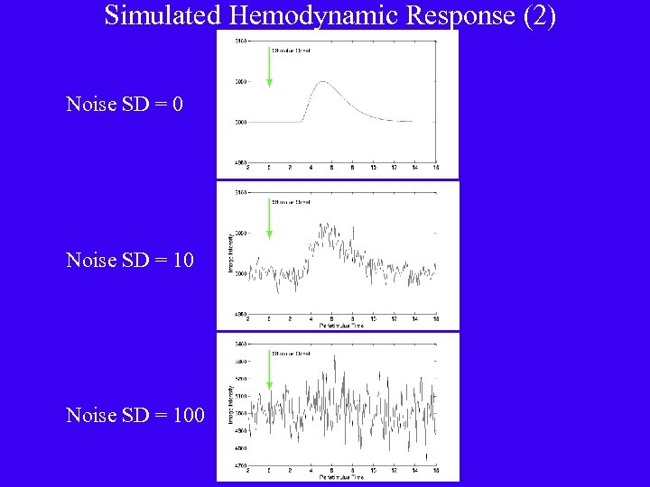
Simulated Hemodynamic Response (2) Noise SD = 0 Noise SD = 100
Event-Related Designs, Two Analyses 1) Using a priori predicted response functions a) long intertrial interval designs b) Reference waveform regression 2) Estimating the actual response a) simple averaging b) Delta Function Regression 3) Some examples
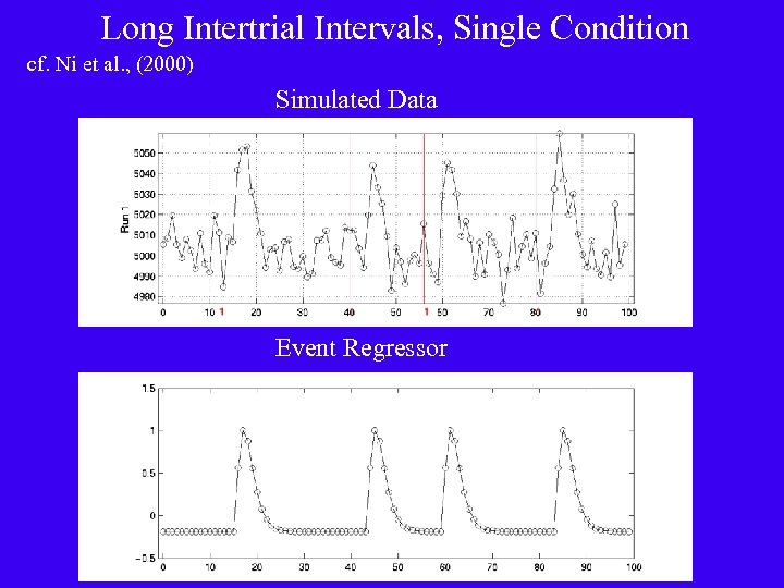
Long Intertrial Intervals, Single Condition cf. Ni et al. , (2000) Simulated Data Event Regressor
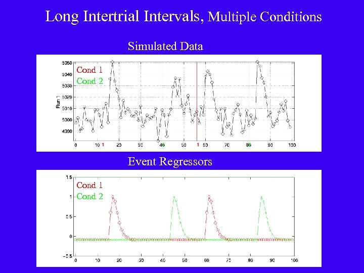
Long Intertrial Intervals, Multiple Conditions Simulated Data Cond 1 Cond 2 Event Regressors Cond 1 Cond 2
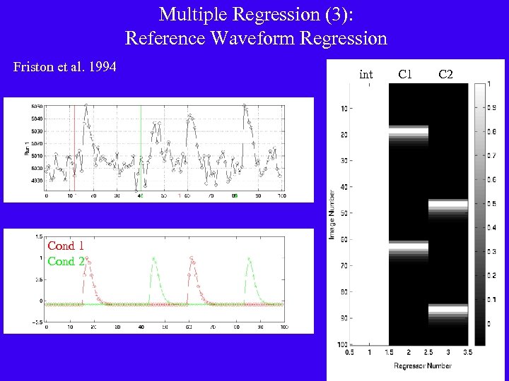
Multiple Regression (3): Reference Waveform Regression Friston et al. 1994 Cond 1 Cond 2 int C 1 C 2
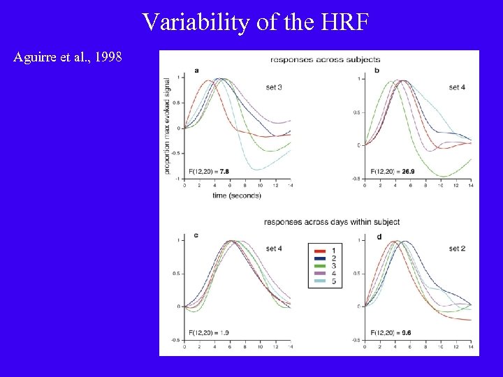
Variability of the HRF Aguirre et al. , 1998
Event-Related Designs, Two Analyses 1) Using a priori predicted response functions a) long intertrial interval designs b) reference waveform regression 2) Estimating the actual response a) simple averaging b) delta function regression 3) Some examples
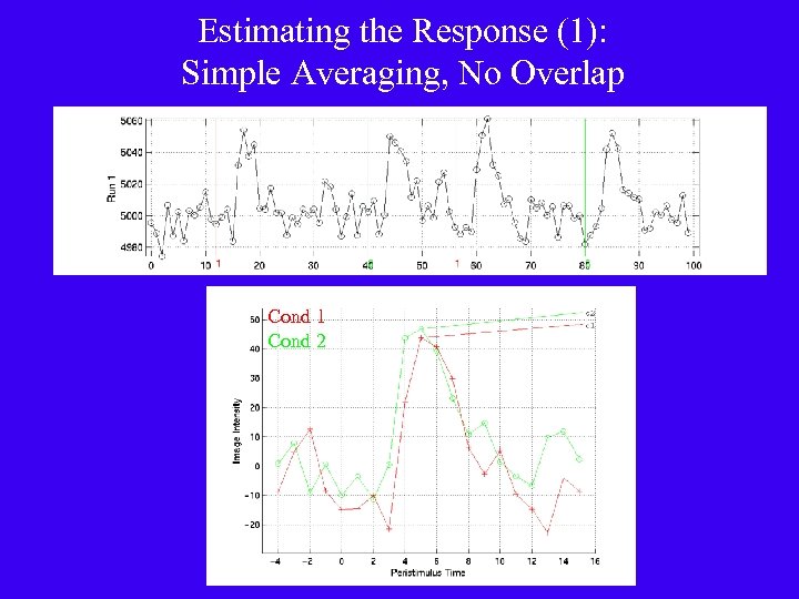
Estimating the Response (1): Simple Averaging, No Overlap Cond 1 Cond 2
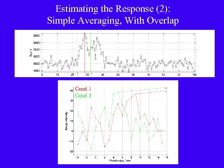
Estimating the Response (2): Simple Averaging, With Overlap Cond 1 Cond 2
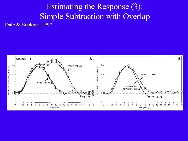
Estimating the Response (3): Simple Subtraction with Overlap Dale & Buckner, 1997
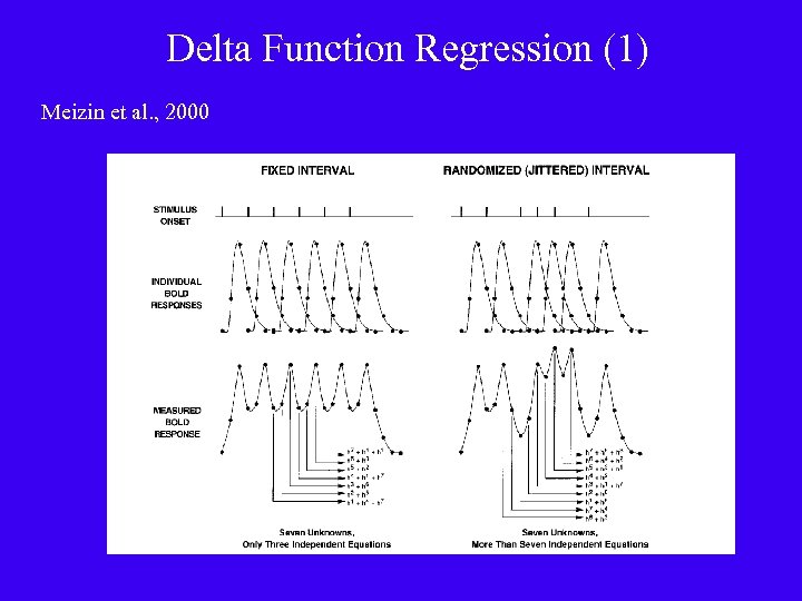
Delta Function Regression (1) Meizin et al. , 2000
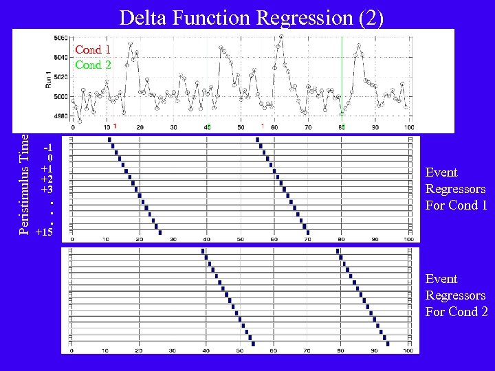
Delta Function Regression (2) Peristimulus Time Cond 1 Cond 2 -1 0 +1 +2 +3. . . +15 Event Regressors For Cond 1 Event Regressors For Cond 2
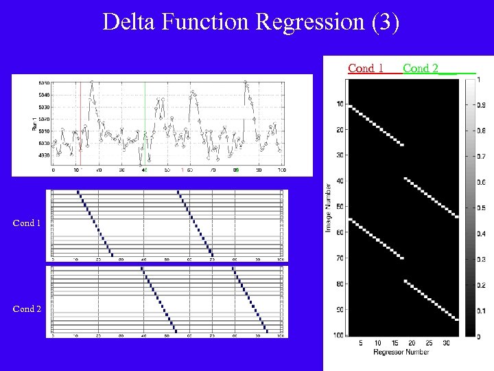
Delta Function Regression (3) Cond 1 Cond 2___
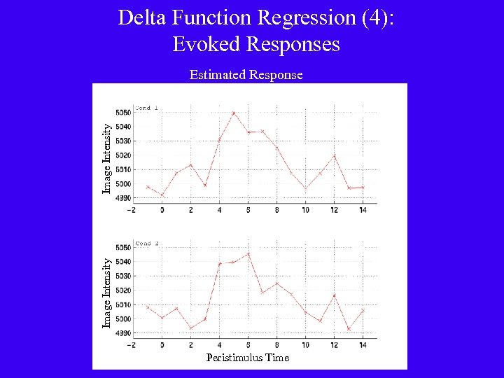
Delta Function Regression (4): Evoked Responses Image Intensity Estimated Response Peristimulus Time
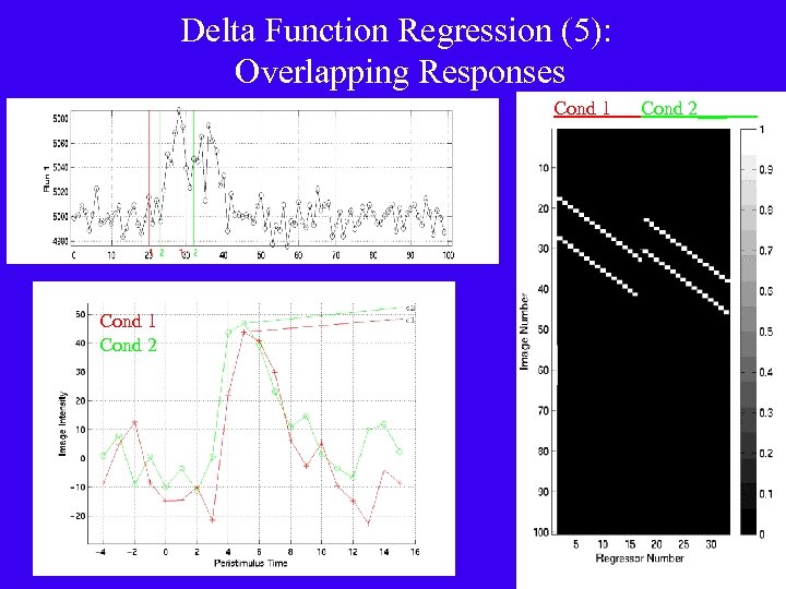
Delta Function Regression (5): Overlapping Responses Cond 1 Cond 2___
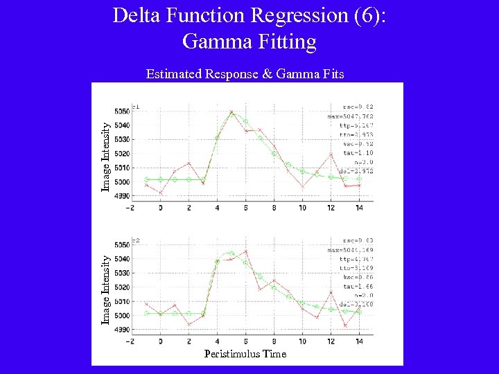
Delta Function Regression (6): Gamma Fitting Image Intensity Estimated Response & Gamma Fits Peristimulus Time
![Delta Function Regression (4): “Blocklet” Analysis Baseline Timepoints [-1 to 0] Activation Timepoints [+3 Delta Function Regression (4): “Blocklet” Analysis Baseline Timepoints [-1 to 0] Activation Timepoints [+3](https://present5.com/presentation/dfacb8289ba7429c2eaf3d0fb7280b5a/image-39.jpg)
Delta Function Regression (4): “Blocklet” Analysis Baseline Timepoints [-1 to 0] Activation Timepoints [+3 to +8] Image Intensity Estimated Response Peristimulus Time
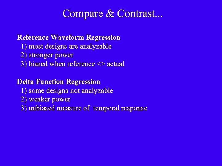
Compare & Contrast. . . Reference Waveform Regression 1) most designs are analyzable 2) stronger power 3) biased when reference <> actual Delta Function Regression 1) some designs not analyzable 2) weaker power 3) unbiased measure of temporal response
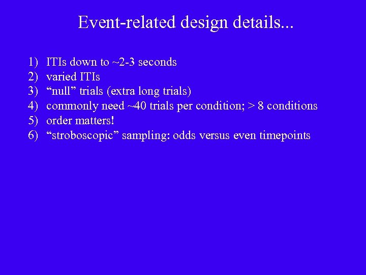
Event-related design details. . . 1) 2) 3) 4) 5) 6) ITIs down to ~2 -3 seconds varied ITIs “null” trials (extra long trials) commonly need ~40 trials per condition; > 8 conditions order matters! “stroboscopic” sampling: odds versus even timepoints
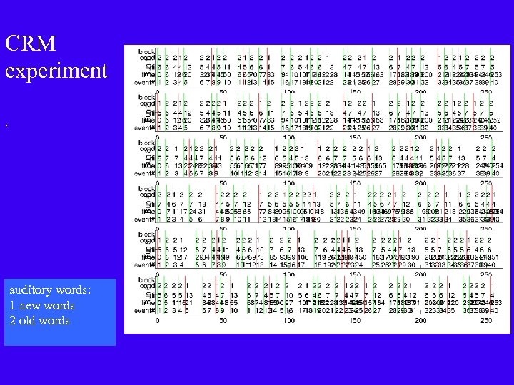
CRM experiment. auditory words: 1 new words 2 old words
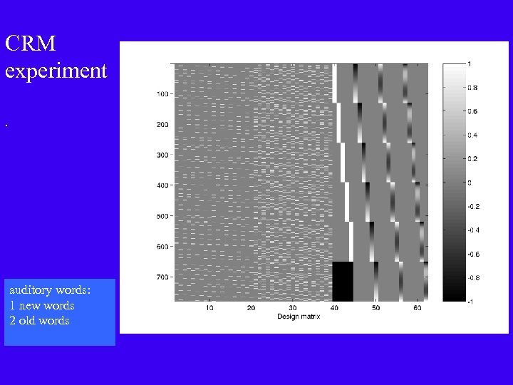
CRM experiment. auditory words: 1 new words 2 old words
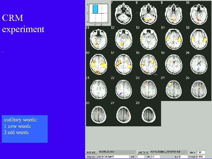
CRM experiment. auditory words: 1 new words 2 old words
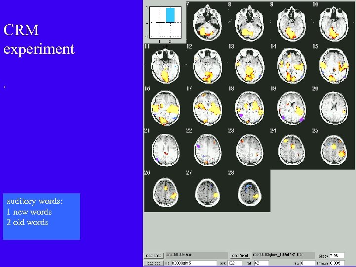
CRM experiment. auditory words: 1 new words 2 old words
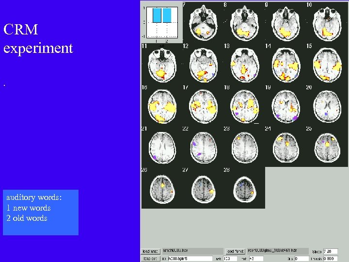
CRM experiment. auditory words: 1 new words 2 old words
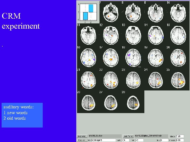
CRM experiment. auditory words: 1 new words 2 old words

CRM experiment. auditory words: 1 new words 2 old words
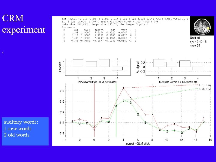
CRM experiment. auditory words: 1 new words 2 old words
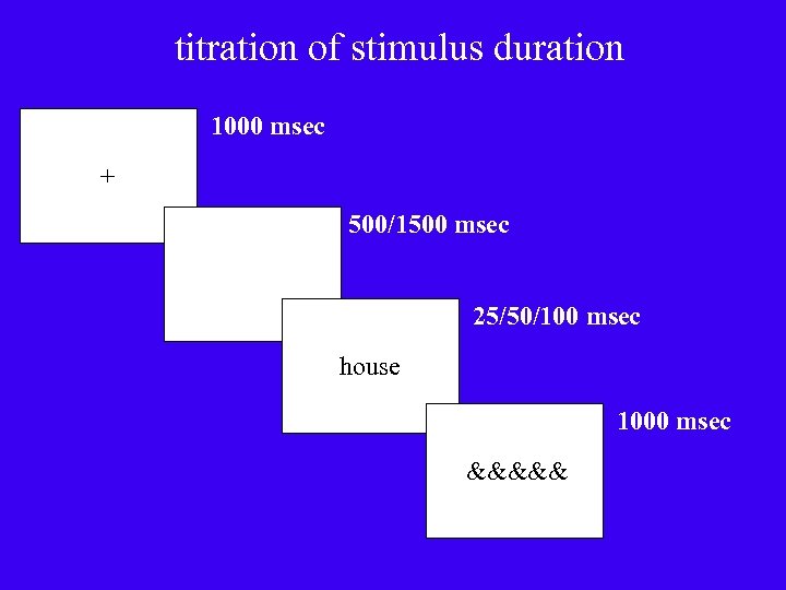
titration of stimulus duration 1000 msec + 500/1500 msec 25/50/100 msec house 1000 msec &&&&&
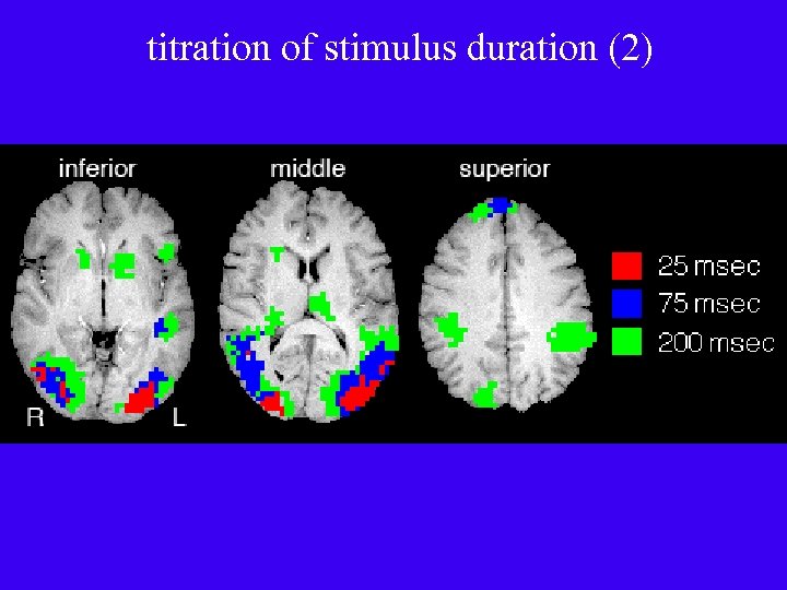
titration of stimulus duration (2)
dfacb8289ba7429c2eaf3d0fb7280b5a.ppt