Growth and Development of Cities Week 4 Urban

Growth and Development of Cities: Week 4. Urban Economy URBS 310 September 14, 2004 1

Urban Growth (O’Sullivan) • • Comparative advantage Scale Economies in Transportation and Trading Cities Internal scale economices Agglomerative economies September 14, 2004 2

Comparative Advantage • • • Trade between regions become advantageous. Trade causes development of cities. Determines whether trade is beneficial or not. Principle of opportunity cost. September 14, 2004 3

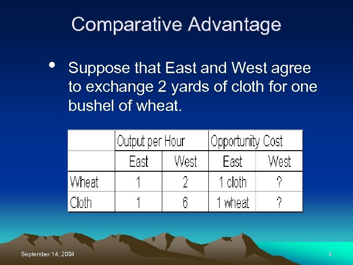
Comparative Advantage • Suppose that East and West agree to exchange 2 yards of cloth for one bushel of wheat. September 14, 2004 4

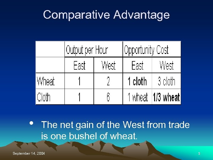
Comparative Advantage • The net gain of the West from trade is one bushel of wheat. September 14, 2004 5

Scale Economies in Transportation • The cost per unit per mile decreases as the volume transported increases. So it is cheaper to transport wheat and cloth in bulk. September 14, 2004 6

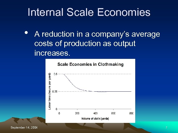
Internal Scale Economies • A reduction in a company’s average costs of production as output increases. September 14, 2004 7

Agglomerative Economies • • • Why are some cities large? By locating close to one another, firms can produce at a lower cost. (positive externality in production: the produdction cost of a particular firm decreases as the production of other firms incraeses). Two types of agglomerative exonomies. September 14, 2004 8

Localization Economies • • The production cost of a particular firm decreases as “industrywide output” increases Three sources – If there are scale economies in the production of an intermediate good, firms share a supplier of an intermediate input and form a cluster around the input supplier. September 14, 2004 9

Localization Economies • Three sources – If output per firm varies from year to year, a cluster of firms facilitates the transfer of workers. (labor market pooling) – A cluster of firms improves communication, rapid exchange of information, and the diffusion of innovations (knowledge spillovers) September 14, 2004 10

Urbanization Economies • • The produdction cost of a particular firm decreases as “total output of the urban area” increases. Result from the sharing of input suppliers (business services & public services), labor-market economies, and communication economies. September 14, 2004 11

Globalization and Urban Growth • • • General Agreement on Trade and Tariffs (GATT)… reduce trade barriers (60% in 30 s, 5% in 70 s). Major effect: manufacturing. Side effect is the weakening of labor unions. What about services? Programming work in India, U. S. hospitals having medical transcription done in India. Insurance claims processing would be candidates for “outsourcing”, “offshoring”. September 14, 2004 12

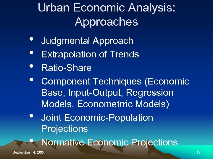
Urban Economic Analysis: Approaches • • • Judgmental Approach Extrapolation of Trends Ratio-Share Component Techniques (Economic Base, Input-Output, Regression Models, Econometrric Models) Joint Economic-Population Projections Normative Economic Projections September 14, 2004 13

Judgmental Approach • • Produces forecasts by polling a panel of experts (Delphi) Used in conjunction with one of technical approaches September 14, 2004 14

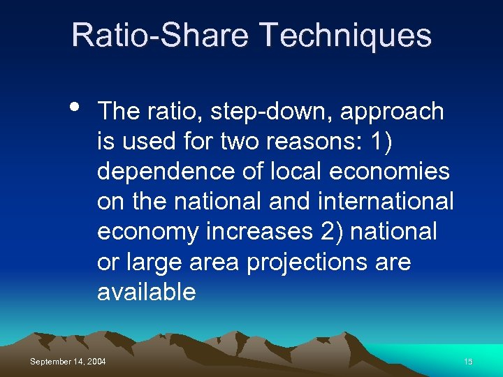
Ratio-Share Techniques • The ratio, step-down, approach is used for two reasons: 1) dependence of local economies on the national and international economy increases 2) national or large area projections are available September 14, 2004 15

Ratio-Share Techniques • Shift-Share Analysis: – 1) the national growth component – 2) national industry shift component – 3) the competitive shift component September 14, 2004 16

Ratio-Share Techniques • Shift-Share Analysis: – 1) the national growth component (N) + – 2) national industry shift component (M) – 3) the competitive shift component (S) September 14, 2004 17

Ratio-Share Techniques • Growth of Movie Industry of LA, 1990 -2000 (MLA 9000): – 1) N = MLA 90 (Tnation 00 / Tnation 90 – 1) + – 2) M = MLA 90 (Mnation 00 / Mnation 90 – – September 14, 2004 Tnation 00 / Tnation 90 ) + 3) S = MLA 90(MLA 00 / MLA 90 – Mnation 00 / Mnation 90 ) 18

Ratio-Share Techniques • Growth of Movie Industry of LA, 1990 -2000 (MLA 9000): – 1) N = MLA 90 (Tnation 00 / Tnation 90 – 1) + – 2) M = MLA 90 (Mnation 00 / Mnation 90 – – September 14, 2004 Tnation 00 / Tnation 90 ) + 3) S = MLA 90(MLA 00 / MLA 90 – Mnation 00 / Mnation 90 ) 19

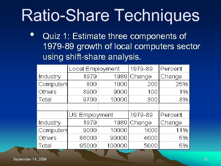
Ratio-Share Techniques • Quiz 1: Estimate three components of 1979 -89 growth of local computers sector using shift-share analysis. September 14, 2004 20

Ratio-Share Techniques • Projection of Movie Industry of LA, 2000 -2010 (MLA 0010): – N = MLA 00 (Mnation 10 / Mnation 00) + – S = MLA 00(MLA 00 / MLA 90 – Mnation 00 / Mnation 90 ) September 14, 2004 21

Ratio-Share Techniques • Assessment – Conceptually and computationally straightforward, easily accessible data, fast and reasonably accurate projections – Instability in the regional (local) competitive component. – The simpler constant shift-share model seems acceptable in many cases. Appropriate for long term baseline forecasts September 14, 2004 22

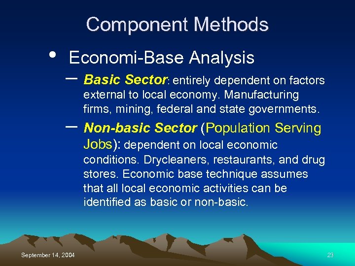
Component Methods • Economi-Base Analysis – Basic Sector: entirely dependent on factors external to local economy. Manufacturing firms, mining, federal and state governments. – Non-basic Sector (Population Serving Jobs): dependent on local economic conditions. Drycleaners, restaurants, and drug stores. Economic base technique assumes that all local economic activities can be identified as basic or non-basic. September 14, 2004 23

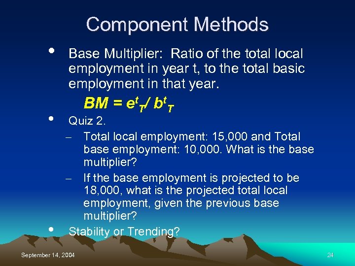
Component Methods • • • Base Multiplier: Ratio of the total local employment in year t, to the total basic employment in that year. BM = et. T/ bt. T Quiz 2. – Total local employment: 15, 000 and Total base employment: 10, 000. What is the base multiplier? – If the base employment is projected to be 18, 000, what is the projected total local employment, given the previous base multiplier? Stability or Trending? September 14, 2004 24

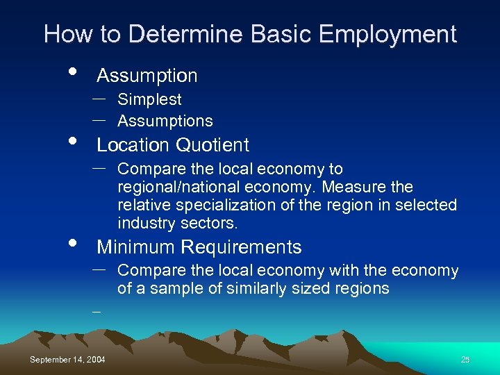
How to Determine Basic Employment • • • Assumption – – Simplest Assumptions Location Quotient – Compare the local economy to regional/national economy. Measure the relative specialization of the region in selected industry sectors. Minimum Requirements – Compare the local economy with the economy of a sample of similarly sized regions – September 14, 2004 25

Location Quotient • • • Developed by Hildebrand Mace (1950) Widely used and Widely criticized Ratio of an industry’s share of the local economy to the industry’s share of the national economy LQi = (eti /et. T ) / (Eti /Et. T ), where eti = regional employment in industry i in year t, et. T = total regional employment in year t, Eti = national employment in industry i in year t, Et. T = total national employment in year t September 14, 2004 26

Location Quotient • • • LQ > 1: the region is more specialized than the nation in the agriculture LQ < 1: the region is less specialized than the nation in the agriculture LQ = 1: the region and the nation specialize to an equal degree in agriculture September 14, 2004 27

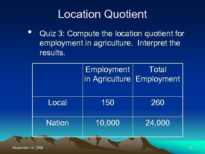
Location Quotient • Quiz 3: Compute the location quotient for employment in agriculture. Interpret the results. Employment Total in Agriculture Employment Local 260 Nation September 14, 2004 150 10, 000 24, 000 28

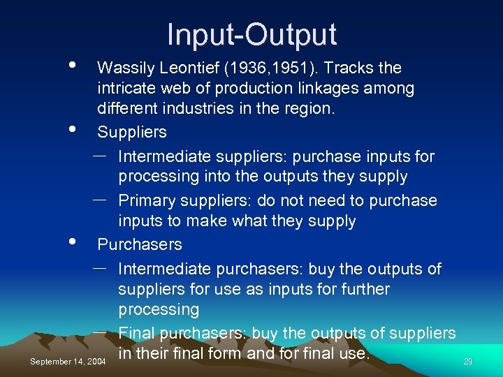
• Input-Output Wassily Leontief (1936, 1951). Tracks the intricate web of production linkages among different industries in the region. • Suppliers – Intermediate suppliers: purchase inputs for processing into the outputs they supply – Primary suppliers: do not need to purchase inputs to make what they supply • Purchasers – Intermediate purchasers: buy the outputs of suppliers for use as inputs for further processing – Final purchasers: buy the outputs of suppliers in their final form and for final use. September 14, 2004 29

Others • • Joint Economic-Population Approach Normative Economic Projection: based on goals and objectives September 14, 2004 30

Sources of Data • • Census Bureau (Dept. of Commerce) Bureau of Labor Statistics ( Dept. of Labor) Bureau of Economic Analysis (Dept. of Commerce) Employment Development Department ( California State) September 14, 2004 31

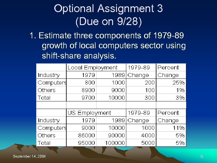
Optional Assignment 3 (Due on 9/28) 1. Estimate three components of 1979 -89 growth of local computers sector using shift-share analysis. September 14, 2004 32

Optional Assignment 3 (Due on 9/28) 2. – Total local employment: 15, 000 and Total base employment: 10, 000. What is the base multiplier? – If the base employment is projected to be 18, 000, what is the projected total local employment, given the previous base multiplier? September 14, 2004 33

Optional Assignment 3 (Due on 9/28) 3. Compute the location quotient for employment in agriculture. Interpret the results. Employment Total in Agriculture Employment Local 260 Nation September 14, 2004 150 10, 000 24, 000 34