70601b5b2d9a15683487579696ab807e.ppt
- Количество слайдов: 45
 Graduate School Quantitative Research Methods Gwilym Pryce Module II Lecture 3: Misspecification: Non-linearities 1
 Summary of Lecture 2: n 1. ANOVA in regression n 2. Prediction n 3. F-Test n 4. Regression assumptions n 5. Properties of OLS estimates 2
 TSS = REGSS + RSS n The sum of squared deviations of y from the mean (i. e. the numerator in the variance of y equation) is called the TOTAL SUM OF SQUARES n The sum of squared deviations of error e is called the RESIDUAL SUM OF SQUARES* * sometimes called the “error sum of squares” n (RSS) The difference between TSS & RSS is called the REGRESSION SUM OF SQUARES# #the n (TSS) (REGSS) REGSS is sometimes called the “explained sum of squares” or “model sum of squares” TSS = REGSS + RSS R 2 = REGSS/ TSS 3
 4. Regression assumptions For estimation of a and b and for regression inference to be correct: n 1. Equation is correctly specified: – – Linear in parameters (can still transform variables) Contains all relevant variables Contains no irrelevant variables Contains no variables with measurement errors n 2. Error Term has zero mean n 3. Error Term has constant variance 4
 n 4. Error Term is not autocorrelated – I. e. correlated with error term from previous time periods n 5. Explanatory variables are fixed – observe normal distribution of y for repeated fixed values of x n 6. No linear relationship between RHS variables – I. e. no “multicolinearity” 5
 5. Properties of OLS estimates n If the above assumptions are met, OLS estimates are said to be BLUE: – Best – Linear – Unbiased I. e. most efficient = least variance – Estimates I. e. estimates of the population parameters. I. e. best amongst linear estimates I. e. in repeated samples, mean of b = b 6
 Plan of Lecture 3: n 1. Consequences of non-linearities n 2. Testing for non-linearities – (a) visual inspection of plots – (b) t-statistics – (c) structural break tests n 3. – – Solutions (a) transform variables (b) split the sample (c) dummies (d) use non-linear estimation techniques 7
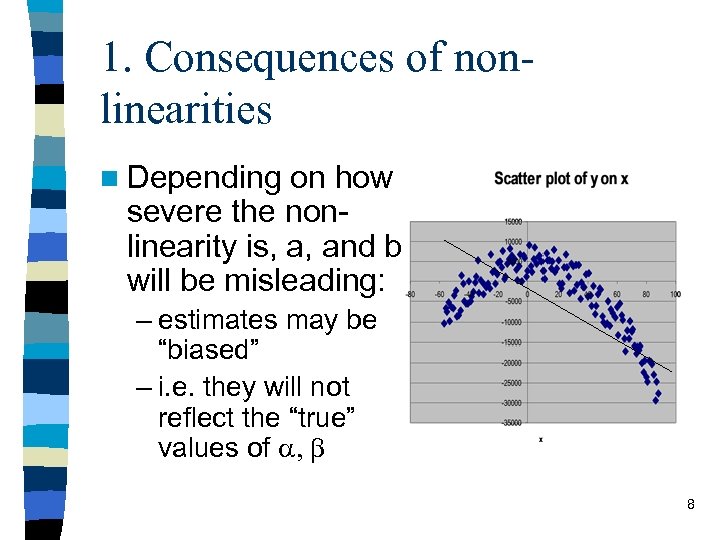 1. Consequences of nonlinearities n Depending on how severe the nonlinearity is, a, and b will be misleading: – estimates may be “biased” – i. e. they will not reflect the “true” values of a, b 8
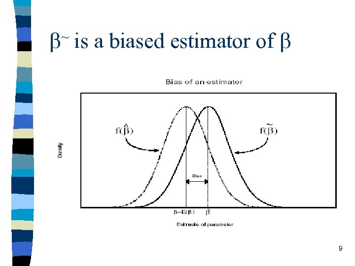 ~ b is a biased estimator of b 9
 2. Testing for non-linearities: (a) visual inspection of plots n scatter plots of two variables: – if you only have two or three variables then looking at scatter plots of these variables can help identify non-linear relationships in the data – but when there are more than 3 variables, non-linearities can be very complex and difficult to identify visually: 10
 – What can appear to be random variation of data points around a linear line of best fit in a 2 -D plot, can turn out to have a systematic cause when a third variable is included and a 3 -D scatter plot is examined. • Same is true when comparing 3 D with higher dimensions • e. g. Suppose that there is a quadratic relationship between x, y and z. But that this is only visible in the data if one controls for the influence of a fourth variable, w. But one does not know this, so looking at x, y and z, they appear to have a linear relationship. 11
 2. Testing for non-linearities: (b) t-statistics n Sometimes variables that we would expect (from intuition or theory) to have a strong effect on the dependent variable turn out to have low t-values. – If so, then one might suspect non-linearities. – Try transforming the variable (e. g. take logs) and re-examine the t-values • e. g. HOUSING DEMAND = a + b AGE OF BORROWER – surprisingly, age of borrower may not be that significant – but this might be because of a non-linearity: housing demand rises with age until mid-life, and starts to decrease as children leave home. Try Age 2 instead and check t-value. 12
 n There may be non-linearities caused by interactions between variables: – try interacting explanatory variables and examining t-values • e. g. HOUSE PRICE = a + b SIZE OF WINDOW + c VIEW • But size of window may only add value to a house if there is a nice view, and having a nice view may only add value if there are windows. • Try including and interactive term as well/instead: – HOUSE PRICE = a +…+ d SIZE OF WINDOW * VIEW • In SPSS you would do this by creating a new variable using the COMPUTE command: – COMPUTE SIZE_VEW = SIZE OF WINDOW * VIEW and then including the new variable in the regression. 13
 2. Testing for non-linearities: (c) shifts & structural break tests n Sometimes certain observations display consistently higher y values. n If this difference can be modelled as a parallel shift of the regression line, then we can incorporate it into our model simply by including an appropriate dummy variable – e. g. male = 1 or 0; 14
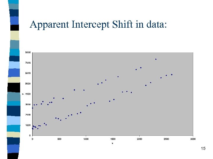 Apparent Intercept Shift in data: 15
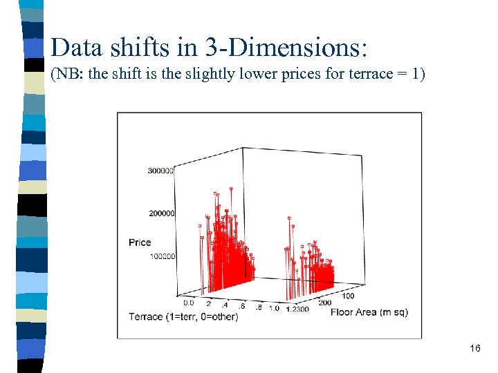 Data shifts in 3 -Dimensions: (NB: the shift is the slightly lower prices for terrace = 1) 16
 n However, sometimes there is an apparent shift in the slope not just/instead of the intercept. n Being able to observe this visually is difficult if you have lots of variables since the visual symptoms will only reveal themselves if the data has been ordered appropriately. 17
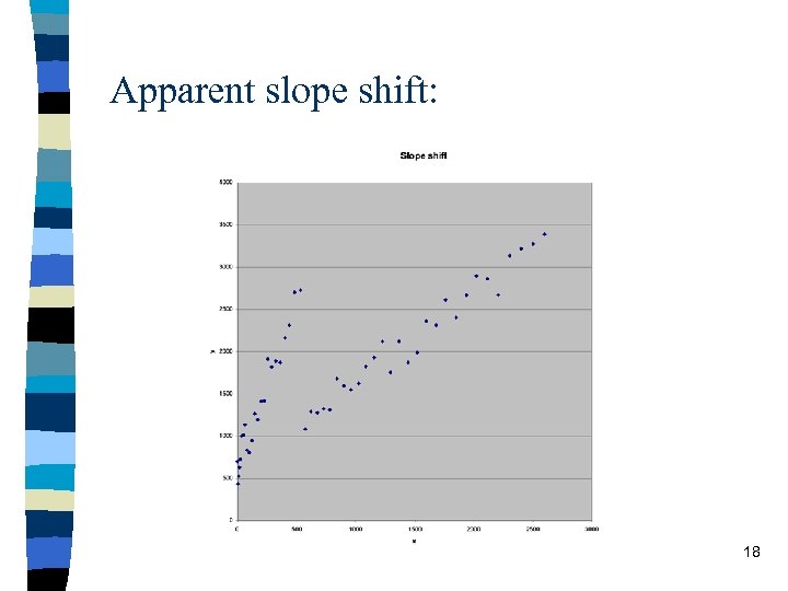 Apparent slope shift: 18
 Solutions: (a) Transforming Variables n Note that “Linear” regression analysis does not preclude analysis of non-linear relationships (a common misconception). – It merely precludes estimation of certain types of non-linear relationships • I. e. those that are non-linear in parameters: • y = ax + az + bxz 19
 n However, so long as the non-linearity can fit within the basic structure of • y = a + bx • I. e. it is linear in parameters – then we can make suitable transformations of the variables and estimate by OLS: 20
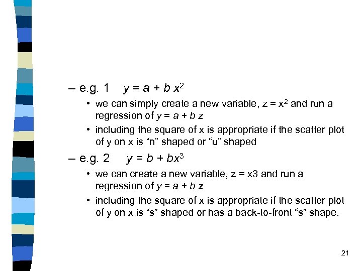 – e. g. 1 y = a + b x 2 • we can simply create a new variable, z = x 2 and run a regression of y = a + b z • including the square of x is appropriate if the scatter plot of y on x is “n” shaped or “u” shaped – e. g. 2 y = b + bx 3 • we can create a new variable, z = x 3 and run a regression of y = a + b z • including the square of x is appropriate if the scatter plot of y on x is “s” shaped or has a back-to-front “s” shape. 21
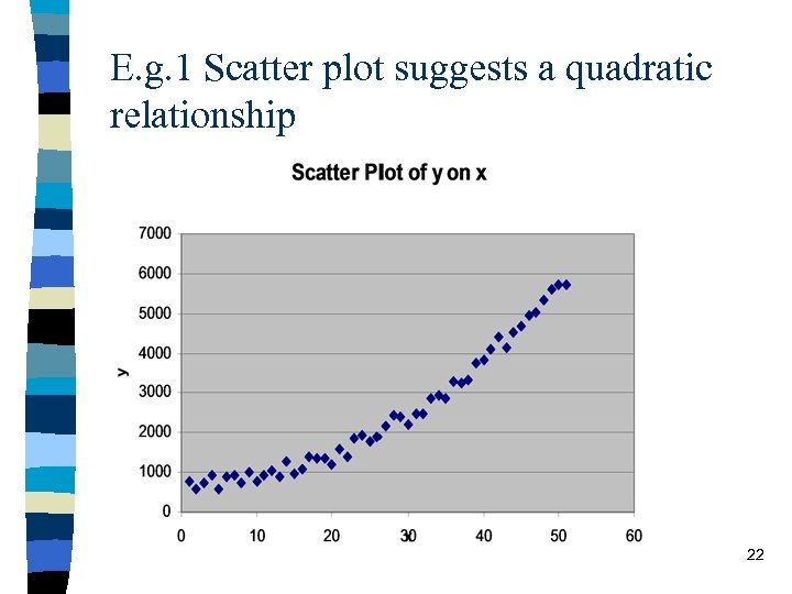 E. g. 1 Scatter plot suggests a quadratic relationship 22
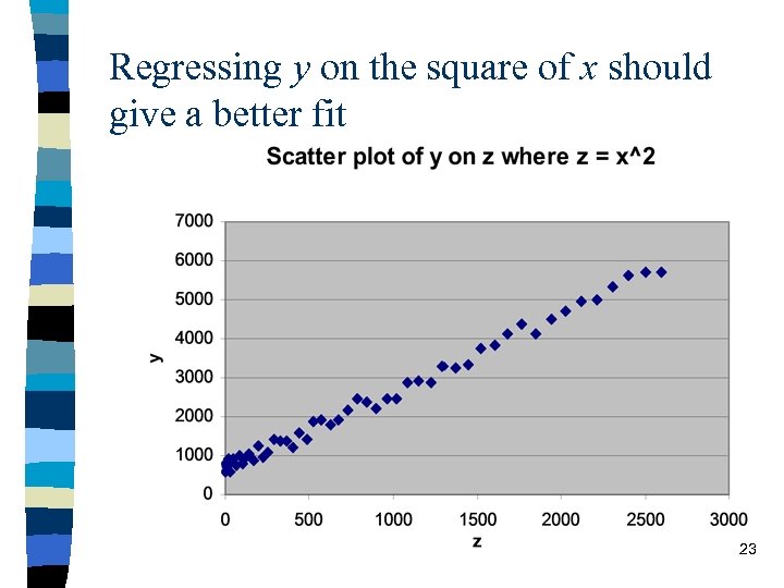 Regressing y on the square of x should give a better fit 23
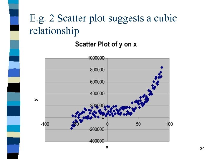 E. g. 2 Scatter plot suggests a cubic relationship 24
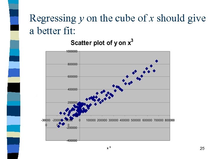 Regressing y on the cube of x should give a better fit: 25
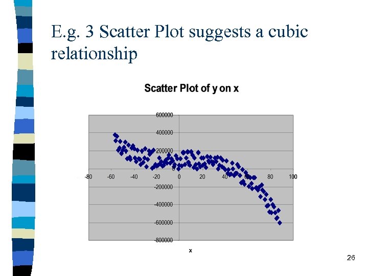 E. g. 3 Scatter Plot suggests a cubic relationship 26
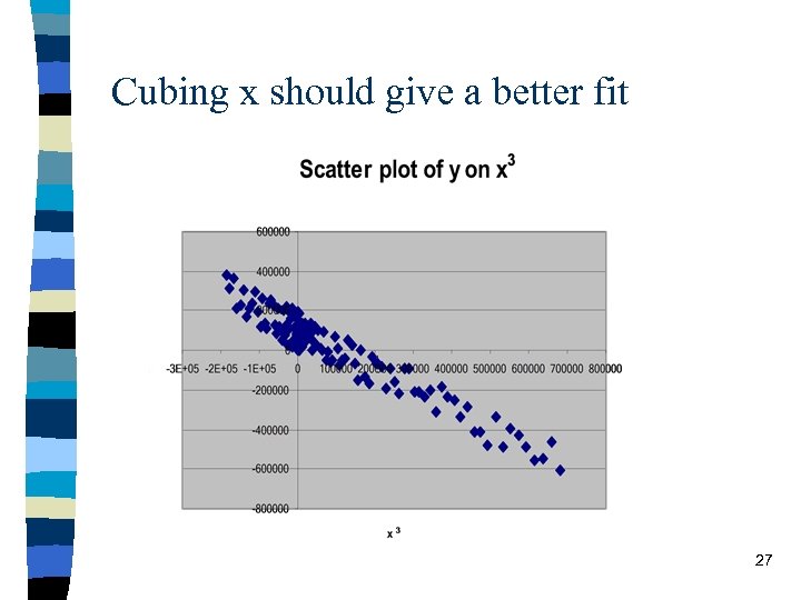 Cubing x should give a better fit 27
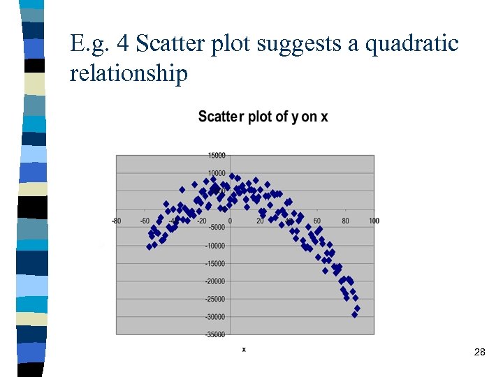 E. g. 4 Scatter plot suggests a quadratic relationship 28
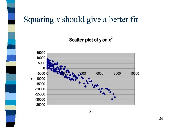 Squaring x should give a better fit 29
 Log-log and log-linear models n One of the most common transformations of either the dependent variable and/or the explanatory variables is to take logs. – It is appropriate to transform x if the scatter plot of y on x has either an “r” shape, or an “L” shape. 30
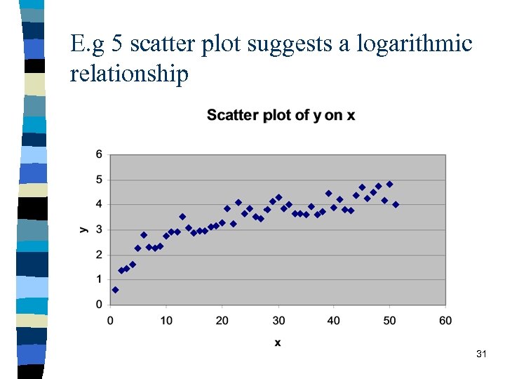 E. g 5 scatter plot suggests a logarithmic relationship 31
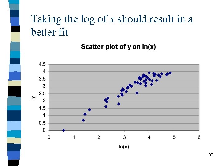 Taking the log of x should result in a better fit 32
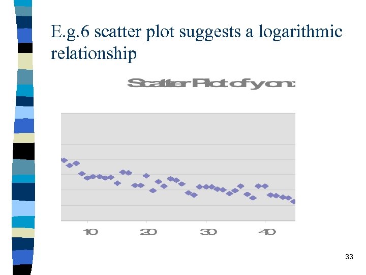 E. g. 6 scatter plot suggests a logarithmic relationship 33
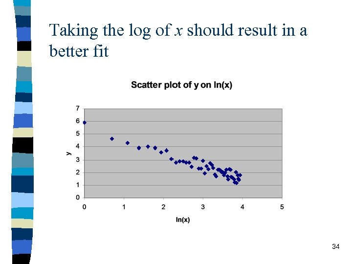 Taking the log of x should result in a better fit 34
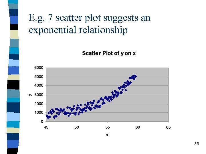 E. g. 7 scatter plot suggests an exponential relationship 35
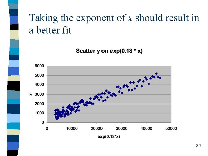 Taking the exponent of x should result in a better fit 36
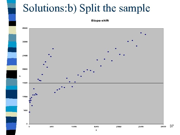 Solutions: b) Split the sample 37
 n Quite a drastic measure: – split the sample and estimate two OLS lines separately – in practice its not easy to decide where exactly to split the sample – we can do an F-test to help us test whethere really is a structural break: “Chow Tests” – but even if the F-test shows that there is a break, it can often be remedied by squaring the offending variable, or using slope dummies. . . 38
 Solutions: (c) Dummy variables n A dummy variable is one that takes the values 0 or 1: – e. g. 1 if male , 0 if female If we include the dummy as a separate variable in the regression we call it an Intercept Dummy n If we multiply it by one of the explanatory variables, then we call it a Slope Dummy n 39
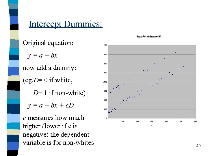 Intercept Dummies: Original equation: y = a + bx now add a dummy: (eg. D= 0 if white, D= 1 if non-white) y = a + bx + c. D c measures how much higher (lower if c is negative) the dependent variable is for non-whites 40
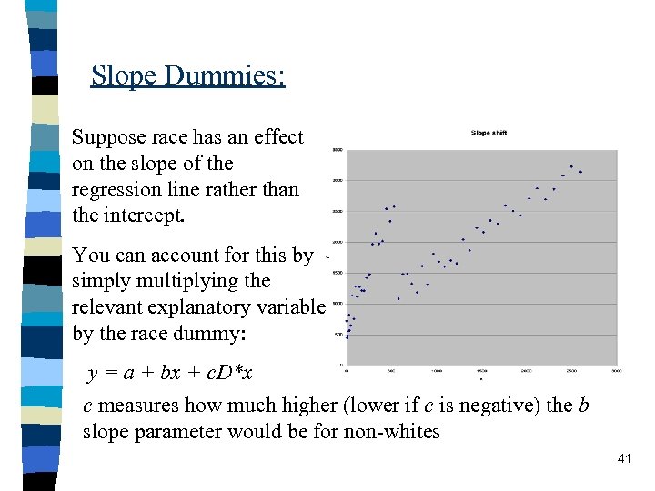 Slope Dummies: Suppose race has an effect on the slope of the regression line rather than the intercept. You can account for this by simply multiplying the relevant explanatory variable by the race dummy: y = a + bx + c. D*x c measures how much higher (lower if c is negative) the b slope parameter would be for non-whites 41
 Solutions: (d) Non-linear estimation When you can’t satisfactorily deal with the non-linearity by simply transforming variables, you can fit a non-linear curve to the data n These are usually based on some sort of grid search (I. e. trial and error) for the correct value of the non-linear parameter. n – E. g. y = a + b 1 eb 2 x + b 3 z • cannot be transformed to linearity in a way that would allow us to derive estimates for b 2 and b 3 42
 n SPSS does allow non-linear estimation – go to Analyse, Regression, non-linear n But we shall not cover this topic in any more detail on this course since most types of non-linearity in data can be adequately dealt with using transformations of the variables. 43
 Summary n 1. Consequences of non-linearities n 2. Testing for non-linearities – (a) visual inspection of plots – (b) t-statistics – (c) structural break tests n 3. – – Solutions (a) transform variables (b) split the sample (c) dummies (d) use non-linear estimation techniques 44
 Reading: n Kennedy (1998) “A Guide to Econometrics”, Chapters 3, 5 and 6 45


