GPGPU Programming Dominik Göddeke Overview Choices

GPGPU Programming Dominik Göddeke

Overview • Choices in GPGPU programming • Illustrated CPU vs. GPU step by step example • GPU kernels in detail 2

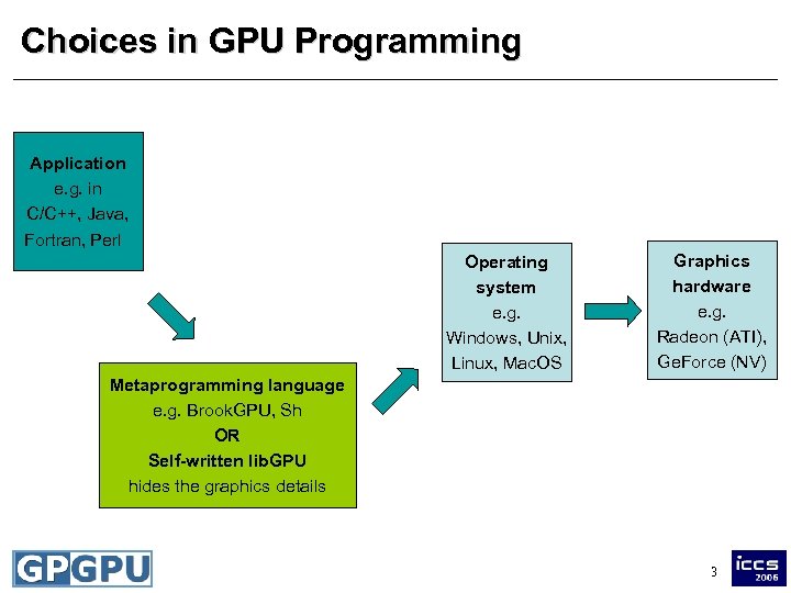Choices in GPU Programming Application e. g. in C/C++, Java, Fortran, Perl Window manager e. g. GLUT, Qt, Win 32, Motif Operating system e. g. Windows, Unix, Linux, Mac. OS Graphics hardware e. g. Radeon (ATI), Ge. Force (NV) Metaprogramming language Shader Graphics API e. g. Brook. GPU, Sh programs e. g. OR e. g. in Open. GL, HLSL, GLSL, Self-written lib. GPU Direct. X Cg hides the graphics details 3

Bottom lines • This is not as difficult as it seems – – Similar choices to be made in all software projects Some options are mutually exclusive Some can be used without in-depth knowledge No direct access to the hardware, the driver does all the tedious thread-management anyway • Advantages and disadvantages – Steeper learning curve vs. higher flexibility – Focus on algorithm, not on (unnecessary) graphics – Portable code vs. platform and hardware specific 4

Libraries and Abstractions • Some coding is required – no library available that you just link against – tremendously hard to massively parallelize existing complex code automatically • Good news – much functionality can be added to applications in a minimally invasive way, no rewrite from scratch • First libraries under development – Accelerator (Microsoft): linear algebra, BLAS-like – Glift (Lefohn et al. ): abstract data structures, e. g. trees 6

Overview • Choices in GPGPU programming • Illustrated CPU vs. GPU step by step example • GPU kernels in detail 7

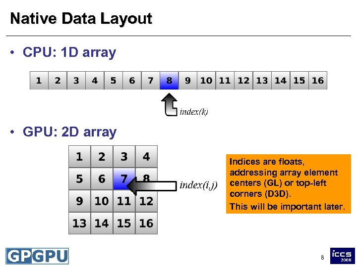Native Data Layout • CPU: 1 D array • GPU: 2 D array Indices are floats, addressing array element centers (GL) or top-left corners (D 3 D). This will be important later. 8

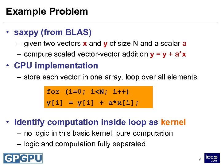Example Problem • saxpy (from BLAS) – given two vectors x and y of size N and a scalar a – compute scaled vector-vector addition y = y + a*x • CPU implementation – store each vector in one array, loop over all elements for (i=0; i

Understanding GPU Limitations • No simultaneous reads and writes into the same memory – No read-modify-write buffer means no logic required to handle read-before-write hazards – Not a missing feature, but essential hardware design for good performance and throughput – saxpy: introduce additional array: ynew = yold + a*x • Coherent memory access – For a given output element, read in from the same index in the two input arrays – Trivially achieved in this basic example 10

Performing Computations • Load a kernel program – Detailed examples later on • Specify the output and input arrays – Pseudocode: set. Input. Arrays(yold, x); set. Output. Array(ynew); • Trigger the computation – GPU is after all a graphics processor – So just draw something appropriate 11

Computing = Drawing • Specify input and output regions – Set up 1: 1 mapping from graphics viewport to output array elements, set up input regions – saxpy: input and output regions coincide • Generate data streams – Literally draw some geometry that covers all elements in the output array – In this example, a 4 x 4 filled quad from four vertices – GPU will interpolate output array indices from vertices across the output region – And generate data stream flowing through the parallel PEs 12

Example Kernel y + 0. 5*x 13

Performing Computations • High-level view – Kernel is executed simultaneously on all elements in the output region – Kernel knows its output index (and eventually additional input indices, more on that later) – Drawing replaces CPU loops, foreach-execution – Output array is write-only • Feedback loop (ping-pong technique) – Output array can be used read-only as input for next operation 14

Overview • Choices in GPGPU programming • Illustrated CPU vs. GPU step by step example • GPU kernels in detail 15

GPU Kernels: saxpy • Kernel on the CPU y[i] = y[i] + a*x[i] • Written in Cg for the GPU float saxpy(float 2 coords: WPOS, uniform sampler. RECT array. X, uniform sampler. RECT array. Y, uniform float a) : COLOR { float y = tex. RECT(array. Y, coords); float x = tex. RECT(array. X, coords); return y+a*x; } array index input arrays gather compute 16

GPU Kernels: Jacobi Iteration • Good news - Simple linear system solver can be built with exactly these basic techniques! • Example: Finite Differences - x: vector of unknowns, sampled with a 5 -point stencil (offsets) - b: right-hand-side - regular, equidistant grid - `solved´ with Jacobi iteration 17

GPU Kernels: Jacobi Iteration calculate offsets float jacobi (float 2 center : WPOS, uniform sampler. RECT x, uniform sampler. RECT b, uniform float one_over_h) : COLOR { float 2 left = center – float 2(1, 0); float 2 right = center + float 2(1, 0); float 2 bottom = center – float 2(0, 1); float 2 top = center + float 2(0, 1); float float gather values = = = tex. RECT(x, tex. RECT(b, center); left); right); bottom); top); center); float Ax = one_over_h * ( 4. 0 * x_center – x_left x_right – x_bottom – x_top ); float inv_diag = one_over_h / 4. 0; matrix-vector Jacobi step x_center x_left x_right x_bottom x_top rhs return x_center + inv_diag * (rhs – Ax); } 18

Maximum of an Array • Entirely different operation – Output is single scalar, input is array of length N • Naive approach – Use 1 x 1 array as output, gather all N values in one step – Doomed: will only use one PE, no parallelism at all – Runs into all sorts of other troubles • Solution: parallel reduction – Idea based on global communication in parallel computing – Smart interplay of output and input regions – Same technique applies to dot products, norms etc. 19

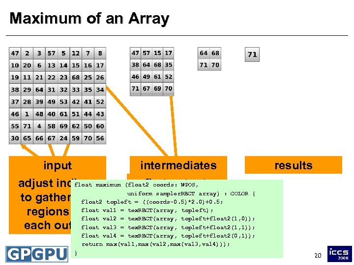Maximum of an Array input intermediates float N/2 x N/2 output input array adjust indicesmaximum (float 2 coords: WPOS, of maximum first output uniform sampler. RECT array) : COLOR { to gather 2 x 2 topleft = ((coords-0. 5)*2. 0)+0. 5; float 2 2 x 2 region float topleft); regions for val 1 = tex. RECT(array, topleft+float 2(1, 0)); float val 2 = tex. RECT(array, float each output val 3 = tex. RECT(array, topleft+float 2(1, 1)); results float val 4 = tex. RECT(array, topleft+float 2(0, 1)); return max(val 1, max(val 2, max(val 3, val 4))); } 20

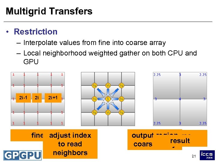Multigrid Transfers • Restriction – Interpolate values from fine into coarse array – Local neighborhood weighted gather on both CPU and GPU 2 i-1 2 i 2 i+1 fine adjust index to read neighbors i output region coarse result coarse array 21

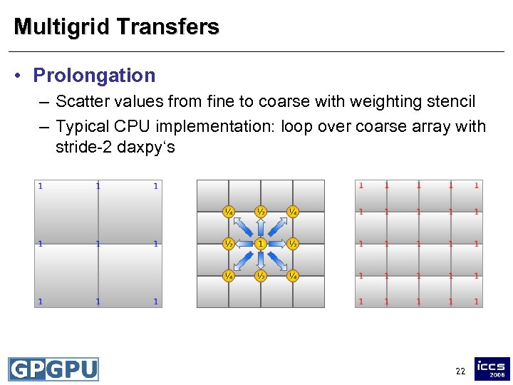Multigrid Transfers • Prolongation – Scatter values from fine to coarse with weighting stencil – Typical CPU implementation: loop over coarse array with stride-2 daxpy‘s 22

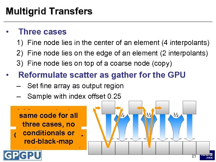Multigrid Transfers • Three cases 1) Fine node lies in the center of an element (4 interpolants) 2) Fine node lies on the edge of an element (2 interpolants) 3) Fine node lies on top of a coarse node (copy) • Reformulate scatter as gather for the GPU – Set fine array as output region – Sample with index offset 0. 25 snaps back to same code for all center (case 3) three cases, no conditionals or 0. 25 snaps to neighred-black-map bors (case 1 and 2) 23

Conclusions • This is not as complicated as it might seem – Course notes online: http: //www. mathematik. uni-dortmund. de/~goeddeke/iccs – GPGPU community site: http: //www. gpgpu. org • Developer information, lots of useful references • Paper archive • Help from real people in the GPGPU forums 24