GOODNESS OF FIT 2 We used OLS

GOODNESS OF FIT

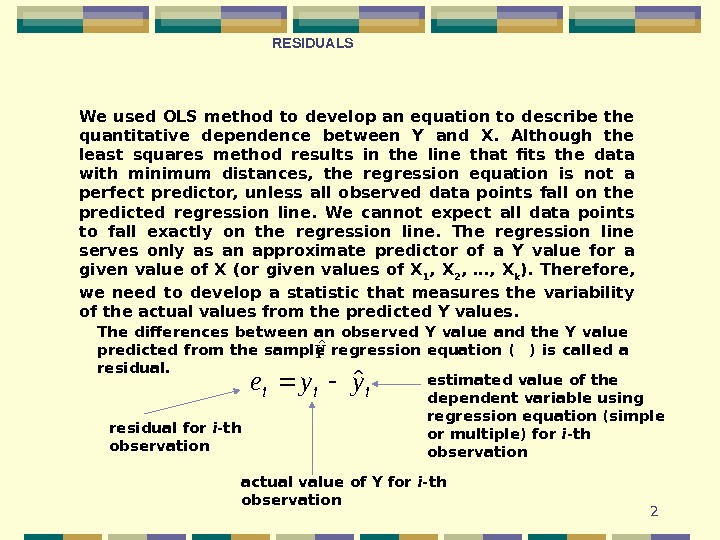
2 We used OLS method to develop an equation to describe the quantitative dependence between Y and X. Although the least squares method results in the line that fits the data with minimum distances, the regression equation is not a perfect predictor, unless all observed data points fall on the predicted regression line. We cannot expect all data points to fall exactly on the regression line. The regression line serves only as an approximate predictor of a Y value for a given value of X (or given values of X 1 , X 2 , …, X k ). Therefore, we need to develop a statistic that measures the variability of the actual values from the predicted Y values. The differences between an observed Y value and the Y value predicted from the sample regression equation ( ) is called a residual. iiiyyeˆ Yˆ residual for i -th observation actual value of Y for i -th observation estimated value of the dependent variable using regression equation (simple or multiple) for i -th observation RESIDUALS

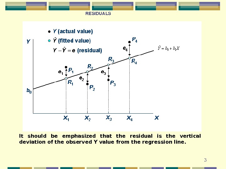
3 It should be emphasized that the residual is the vertical deviation of the observed Y value from the regression line. RESIDUALS

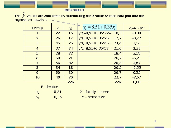
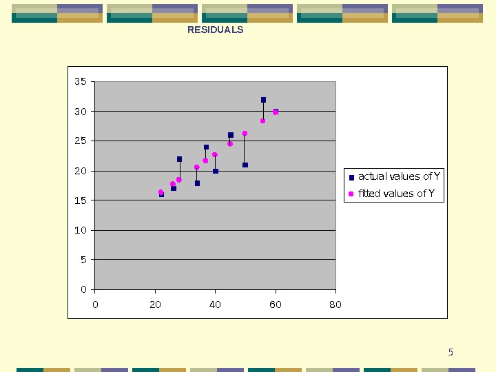
4 Familyxiyiei=yi — y^i 12216 y^1=8, 51+0, 35*22=16, 3 -0, 30 22617 y^2=8, 51+0, 35*26=17, 7 -0, 72 34526 y^3=8, 51+0, 35*45=24, 41, 56 43724 y^4=8, 51+0, 35*37=21, 62, 39 5282218, 43, 58 6502126, 2 -5, 21 7563228, 33, 67 8341820, 5 -2, 55 9603029, 70, 25 10402022, 7 -2, 67 2262260, 00 b 08, 51 X — family income b 10, 35 Y — home size Estimators. The values are calculated by substituting the X value of each data pair into the regression equation. y ˆ RESIDUALS

505101520253035 0 20 40 60 80 actual values of Y fitted values of YRESIDUALS

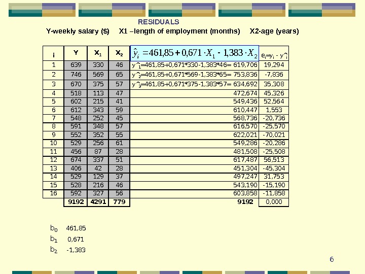
6 Y- weekly salary ($) X 1 – length of employment (month s) X 2 — age (years )i. YX 1 X 2 ei=yi — y^i 163933046619, 70619, 294 274656965753, 836 -7, 836 367037557634, 69235, 308 451811347472, 67445, 326 560221541549, 43652, 564 661234359610, 4471, 553 754825245568, 736 -20, 736 859134857616, 570 -25, 570 955235255622, 021 -70, 021 1052925661549, 286 -20, 286 114568728481, 508 -25, 508 1267433751617, 48756, 513 134064228451, 304 -45, 304 1452912937497, 24731, 753 1552821646543, 190 -15, 190 1659232756603, 858 -11, 858 9192429177991920, 000 b 0461, 85 b 10, 671 b 2 -1, 383 y^1=461, 85+0, 671*330 -1, 383*46= y^2=461, 85+0, 671*569 -1, 383*65= y^3=461, 85+0, 671*375 -1, 383*57=RESIDUALS 21383, 1671, 085, 461ˆXXyi

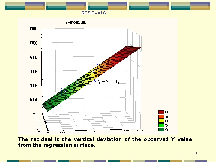
7 Y = 461, 85+0, 671*X 1 -1, 383 X 2 800 700 600 500 400 iiiyyeˆThe residual is the vertical deviation of the observed Y value from the regression surface. RESIDUALS

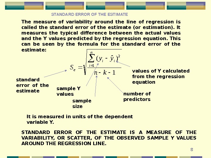
8 The measure of variability around the line of regression is called the standard error of the estimate (or estimation). It measures the typical difference between the actual values and the Y values predicted by the regression equation. This can be seen by the formula for the standard error of the estimate: 1 )ˆ( 1 2 kn yy S n i ii e standard error of the estimate sample Y values of Y calculated from the regression equation sample size number of predictors It is measured in units of the dependent variable Y. STANDARD ERROR OF THE ESTIMATE IS A MEASURE OF THE VARIABILITY, OR SCATTER, OF THE OBSERVED SAMPLE Y VALUES AROUND THE REGRESSION LINE. STANDARD ERROR OF THE ESTIMAT

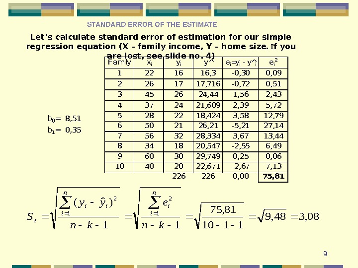
9 Let’s calculate standard error of estimation for our simple regression equation (X – family income, Y – home size. I f you are lost, see slide no. 4)Familyxiyiei=yi — y^iei 2 1221616, 3 -0, 300, 09 2261717, 716 -0, 720, 51 3452624, 441, 562, 43 4372421, 6092, 395, 72 5282218, 4243, 5812, 79 6502126, 21 -5, 2127, 14 7563228, 3343, 6713, 44 8341820, 547 -2, 556, 49 9603029, 7490, 250, 06 10402022, 671 -2, 677, 13 2262260, 0075, 81 y^ 08, 348, 9 1110 81, 75 11 )ˆ( 1 2 kn e kn yy S n i ii e b 0=8, 51 b 1=0, 35 STANDARD ERROR OF THE ESTIMAT

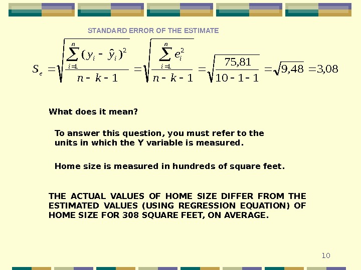
1008, 348, 9 1110 81, 75 11 )ˆ( 1 2 kn e kn yy S n i ii e. THE ACTUAL VALUES OF HOME SIZE DIFFER FROM THE ESTIMATED VALUES (USING REGRESSION EQUATION) OF HOME SIZE FOR 308 SQUARE FEET, ON AVERAGE. What does it mean? To answer this question, you must refer to the units in which the Y variable is measured. Home size is measured in hundreds of square feet. STANDARD ERROR OF THE ESTIMAT

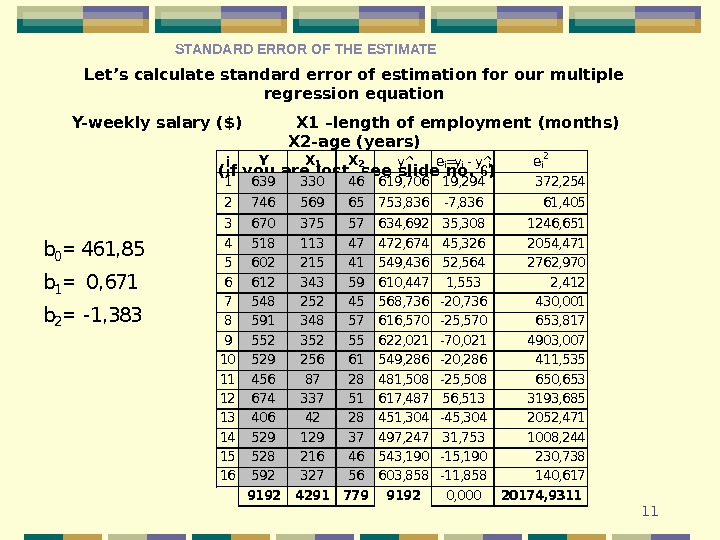
11 Let’s calculate standard error of estimation for our multiple regression equation Y- weekly salary ($) X 1 – length of employment (month s) X 2 — age (years ) ( i f you are lost, see slide no. 6 )i. YX 1 X 2 ei=yi — y^iei 2 163933046619, 70619, 294372, 254 274656965753, 836 -7, 83661, 405 367037557634, 69235, 3081246, 651 451811347472, 67445, 3262054, 471 560221541549, 43652, 5642762, 970 661234359610, 4471, 5532, 412 754825245568, 736 -20, 736430, 001 859134857616, 570 -25, 570653, 817 955235255622, 021 -70, 0214903, 007 1052925661549, 286 -20, 286411, 535 114568728481, 508 -25, 508650, 653 1267433751617, 48756, 5133193, 685 134064228451, 304 -45, 3042052, 471 1452912937497, 24731, 7531008, 244 1552821646543, 190 -15, 190230, 738 1659232756603, 858 -11, 858140, 617 9192429177991920, 00020174, 9311 y^ b 0=461, 85 b 1=0, 671 b 2=-1, 383 STANDARD ERROR OF THE ESTIMAT

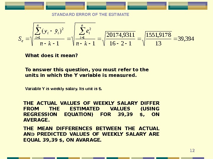
12394, 39 13 9178, 1551 1216 9311, 20174 11 )ˆ(1 2 kn e kn yy S n i ii e What does it mean? To answer this question, you must refer to the units in which the Y variable is measured. THE ACTUAL VALUES OF WEEKLY SALARY DIFFER FROM THE ESTIMATED VALUES (USING REGRESSION EQUATION) FOR 39, 39 $ , ON AVERAGE. THE MEAN DIFFERENCES BETWEEN THE ACTUAL AN D PREDICTED VALUES OF WEEKLY SALARY ARE EQUAL 39, 39 $, ON AVARAGE. Variable Y is weekly salary. Its unit is $. STANDARD ERROR OF THE ESTIMAT

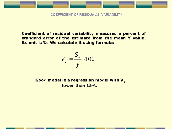
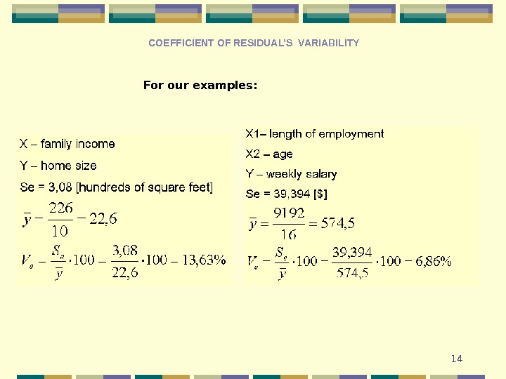
13 COEFFICIENT OF RESIDUAL’S VARIABILITY Coefficient of residual variability measures a percent of standard error of the estimate from the mean Y value. Its unit is %. We calculate it using formula: 100 y S V e e Good model is a regression model with V e lower than 15%.

14 For our examples: COEFFICIENT OF RESIDUAL’S VARIABILITY

15 HOW GOOD IS OUR MODEL? In order to examine how well the independent variable (or variables) predicts the dependent variable in our model, we need to develop several measures of variation. The first measure, the TOTAL SUM OF SQUARES (SST), is a measure of variation (or scatter) of the Y values around the mean. The total sum of squares can be subdivided into explained variation (or REGRESSION SUM OF SQUARES, SSR), that is attributable to the relationship between the independent variable (or variables) and the dependent variable, and unexplained variation (or ERROR SUM OF SQUARES, SSE), that which is attributable to factors other than the relationship between the independent variable (or variables) and the dependent variable.

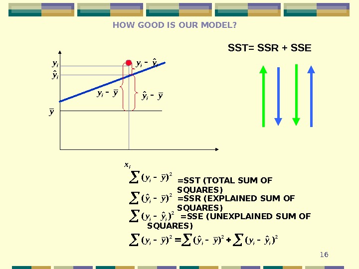
16 HOW GOOD IS OUR MODEL? SST= SSR + SSEy ix iy iyˆ yyiyyiˆ iiyyˆ 2 )( yy i =SST ( TOTAL SUM OF SQUARES) 2 )ˆ ( yy i =SSR ( EXPLAINED SUM OF SQUARES) 2 )ˆ ( ii yy =SSE ( UNEXPLAINED SUM OF SQUARES) 222 )ˆ ()( iiii yyyyyy

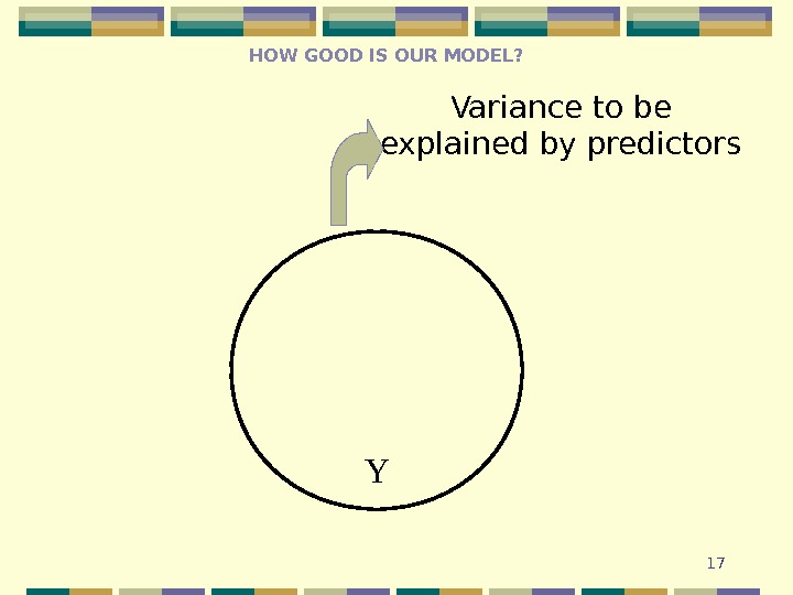
17 Y Variance to be explained by predictors. HOW GOOD IS OUR MODEL?

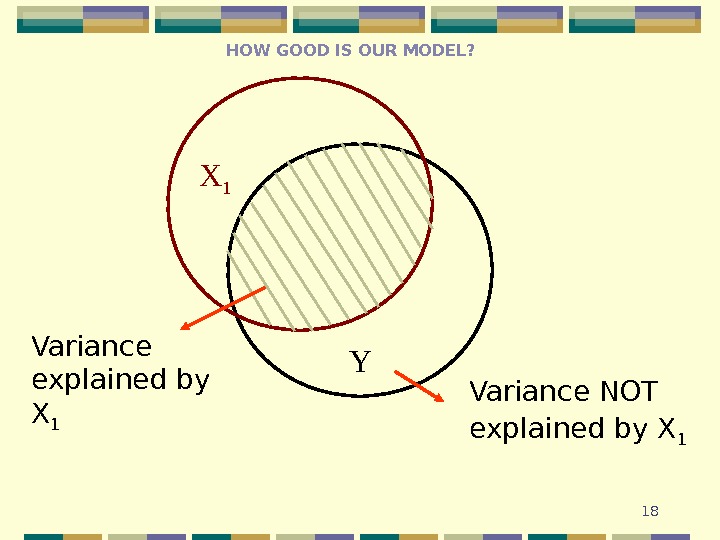
18 YX 1 Variance NOT explained by X 1 Variance explained by X 1 HOW GOOD IS OUR MODEL?

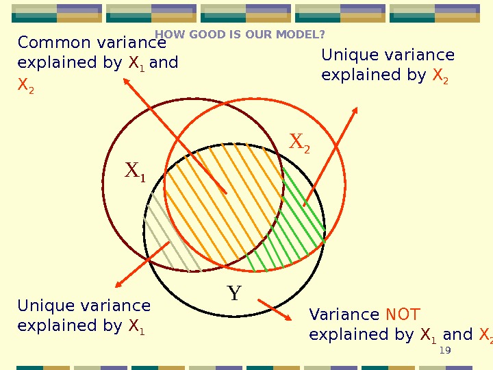
19 YX 1 Variance NOT explained by X 1 and X 2 Unique variance explained by X 1 Unique variance explained by X 2 Common variance explained by X 1 and X 2 HOW GOOD IS OUR MODEL?

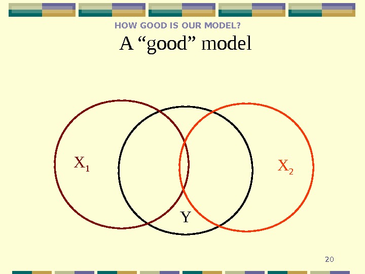
20 YX 1 X 2 A “good” model. HOW GOOD IS OUR MODEL?

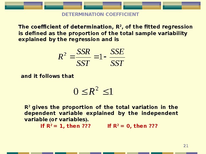
21 The coefficient of determination, RR 22 , of the fitted regression is defined as the proportion of the total sample variability explained by the regression and is. SST SSE SST SSR R 1 2 DETERMINATION COEFFICIENT and it follows that 10 2 R R 2 gives the proportion of the total variation in the dependent variable explained by the independent variable ( or variables ). If R 2 = 1, then ? ? ? If R 2 = 0 , then ? ? ?

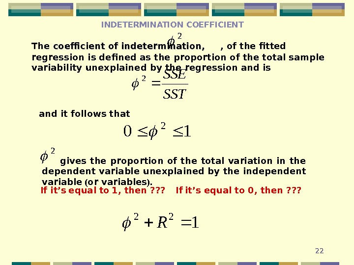
22 INDETERMINATION COEFFICIENT The coefficient of indetermination , , , of the fitted regression is defined as the proportion of the total sample variability unexplained by the regression and is. SST SSE 2 and it follows that 10 2 gives the proportion of the total variation in the dependent variable unexplained by the independent variable ( or variables ). 2 If it’s equal to 1, then ? ? ? If it’s equal to 0 , then ? ? ? 2 1 22 R

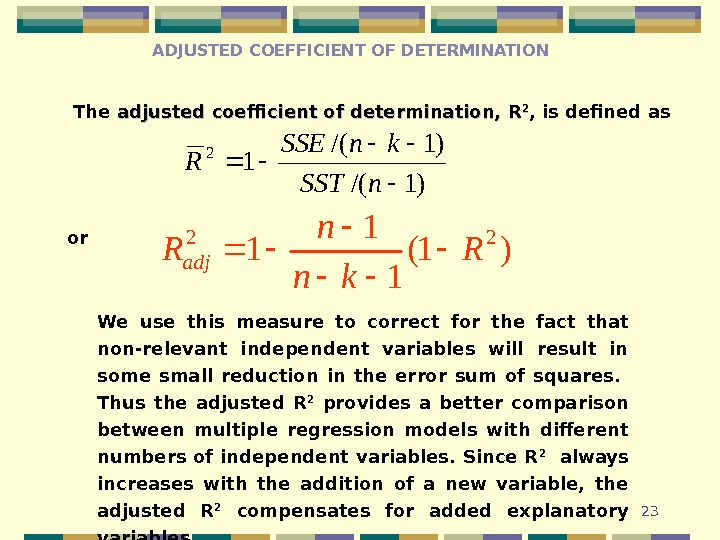
23 ADJUSTED COEFFICIENT OF DETERMINATION The adjusted coefficient of determination, RR 22 , is defined as )1/( 12 n. SST kn. SSE R We use this measure to correct for the fact that non-relevant independent variables will result in some small reduction in the error sum of squares. Thus the adjusted R 2 provides a better comparison between multiple regression models with different numbers of independent variables. Since R 2 always increases with the addition of a new variable, the adjusted R 2 compensates for added explanatory variables. )1( 1 1 1 22 R kn n Radj or

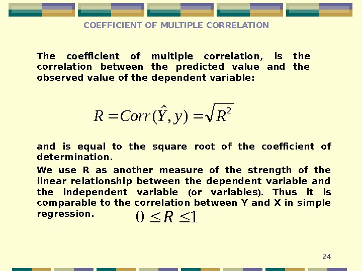
24 COEFFICIENT OF MULTIPLE CORRELATION The coefficient of multiple correlation , is the correlation between the predicted value and the observed value of the dependent variable : 2 ), ˆ ( Ry. YCorr. R and is equal to the square root of the coefficient of determination. We use R as another measure of the strength of the linear relationship between the dependent variable and the independent variable ( or variables ). Thus it is comparable to the correlation between Y and X in simple regression. 10 R

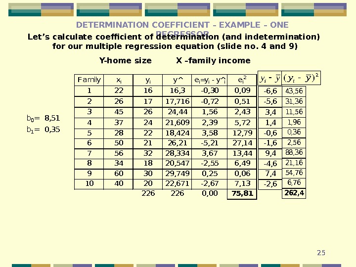
25 DETERMINATION COEFFICIENT – EXAMPLE – ONE REGRESSOR Let’s calculate coefficient of determination (and indetermination) for our multiple regression equation ( slide no. 4 and 9 ) Y-home size X –family incomeb 0=8, 51 b 1=0, 35 Familyxiyiei=yi — y^iei 2 1221616, 3 -0, 300, 09 2261717, 716 -0, 720, 51 3452624, 441, 562, 43 4372421, 6092, 395, 72 5282218, 4243, 5812, 79 6502126, 21 -5, 2127, 14 7563228, 3343, 6713, 44 8341820, 547 -2, 556, 49 9603029, 7490, 250, 06 10402022, 671 -2, 677, 13 2262260, 0075, 81 y^ -6, 6 -5, 6 3, 4 1, 4 -0, 6 -1, 6 9, 4 -4, 6 7, 4 -2, 6 43, 56 31, 36 11, 56 1, 96 0, 36 2, 56 88, 36 21, 16 54, 76 6, 76 262, 4 yyi 2)(yyi

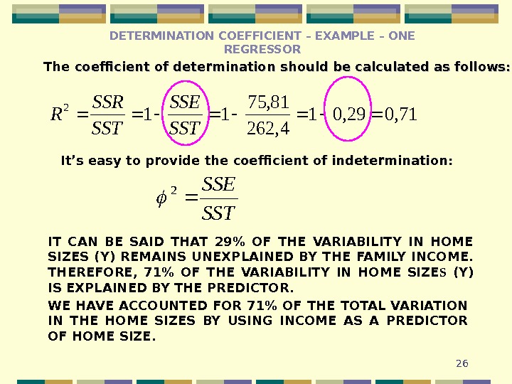
26 The coefficient of determination should be calculated as follows: 71, 029, 01 4, 262 81, 75 112 SST SSE SST SSR R It’s easy to provide the coefficient of inin determination : : SST SSE 2 IT CAN BE SAID THAT 29% OF THE VARIABILITY IN HOME SIZES (Y) REMAINS UNEXPLAINED BY THE FAMILY INCOME. THEREFORE, 71% OF THE VARIABILITY IN HOME SIZE S (Y) IS EXPLAINED BY THE PREDICTOR. WE HAVE ACCOUNTED FOR 71% OF THE TOTAL VARIATION IN THE HOME SIZES BY USING INCOME AS A PREDICTOR OF HOME SIZE. DETERMINATION COEFFICIENT – EXAMPLE – ONE REGRESSOR

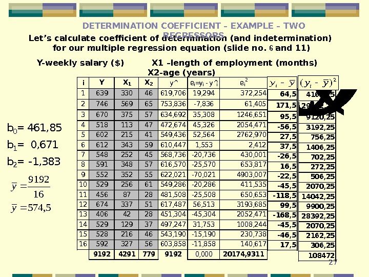
27 Let’s calculate coefficient of determination (and indetermination) for our multiple regression equation ( slide no. 6 and 11 ) Y- weekly salary ($) X 1 – length of employment (month s) X 2 — age (years )i. YX 1 X 2 ei=yi — y^iei 2 163933046619, 70619, 294372, 254 274656965753, 836 -7, 83661, 405 367037557634, 69235, 3081246, 651 451811347472, 67445, 3262054, 471 560221541549, 43652, 5642762, 970 661234359610, 4471, 5532, 412 754825245568, 736 -20, 736430, 001 859134857616, 570 -25, 570653, 817 955235255622, 021 -70, 0214903, 007 1052925661549, 286 -20, 286411, 535 114568728481, 508 -25, 508650, 653 1267433751617, 48756, 5133193, 685 134064228451, 304 -45, 3042052, 471 1452912937497, 24731, 7531008, 244 1552821646543, 190 -15, 190230, 738 1659232756603, 858 -11, 858140, 617 9192429177991920, 00020174, 9311 y^ b 0=461, 85 b 1=0, 671 b 2=-1, 383 5, 574 16 9192 y y 64, 5 171, 5 95, 5 -56, 5 27, 5 37, 5 -26, 5 16, 5 -22, 5 -45, 5 -118, 5 99, 5 -168, 5 -45, 5 -46, 5 17, 5 4160, 25 29412, 25 9120, 25 3192, 25 756, 25 1406, 25 702, 25 272, 25 506, 25 2070, 25 14042, 25 9900, 25 28392, 25 2070, 25 2162, 25 306, 25 108472 2)(yyiyyi 2)(yyi. DETERMINATION COEFFICIENT – EXAMPLE – TWO REGRESSORS

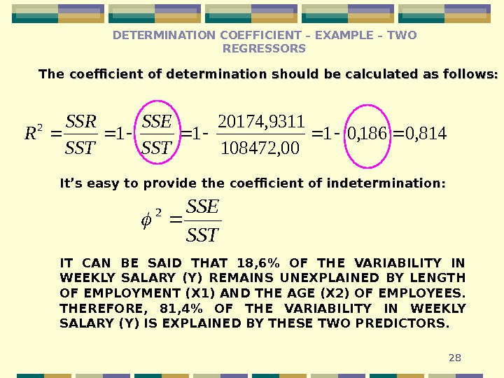
28814, 0186, 01 00, 108472 9311, 20174 11 2 SST SSE SST SSR RThe coefficient of determination should be calculated as follows: It’s easy to provide the coefficient of inin determination : : SST SSE 2 IT CAN BE SAID THAT 18, 6% OF THE VARIABILITY IN WEEKLY SALARY (Y) REMAINS UNEXPLAINED BY LENGTH OF EMPLOYMENT (X 1) AND THE AGE (X 2) OF EMPLOYEES. THEREFORE, 81, 4% OF THE VARIABILITY IN WEEKLY SALARY (Y) IS EXPLAINED BY THESE TWO PREDICTORS. DETERMINATION COEFFICIENT – EXAMPLE – TWO REGRESSORS

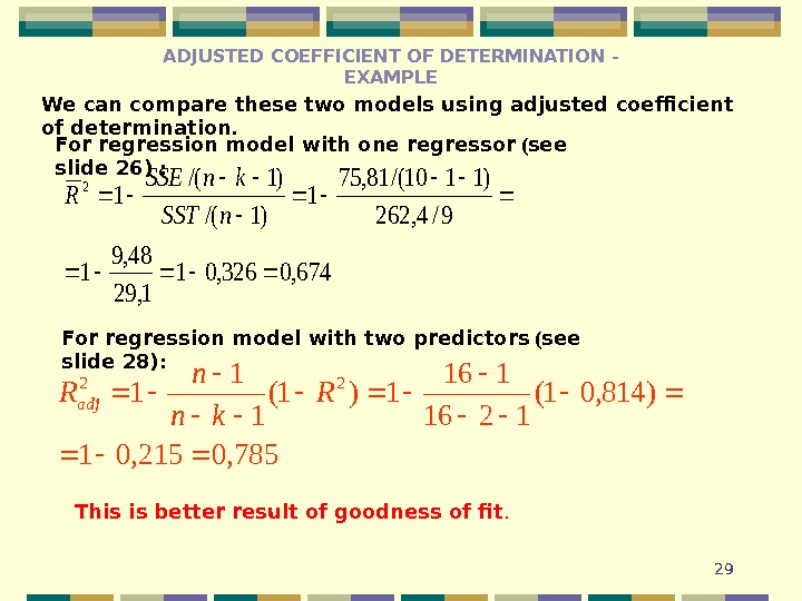
29 We can compare these two models using adjusted coefficient of determination. For regression model with one regressor ( see slide 26) : For regression model with two predictors ( see slide 28) : 674, 0326, 01 1, 29 48, 9 1 9/4, 262 )1110/(81, 75 1 )1/( 1 2 n. SST kn. SSE R 785, 0215, 01 )814, 01( 1216 1)1( 1 1 1 22 R kn n Radj This is better result of goodness of fit. ADJUSTED COEFFICIENT OF DETERMINATION — EXAMPL

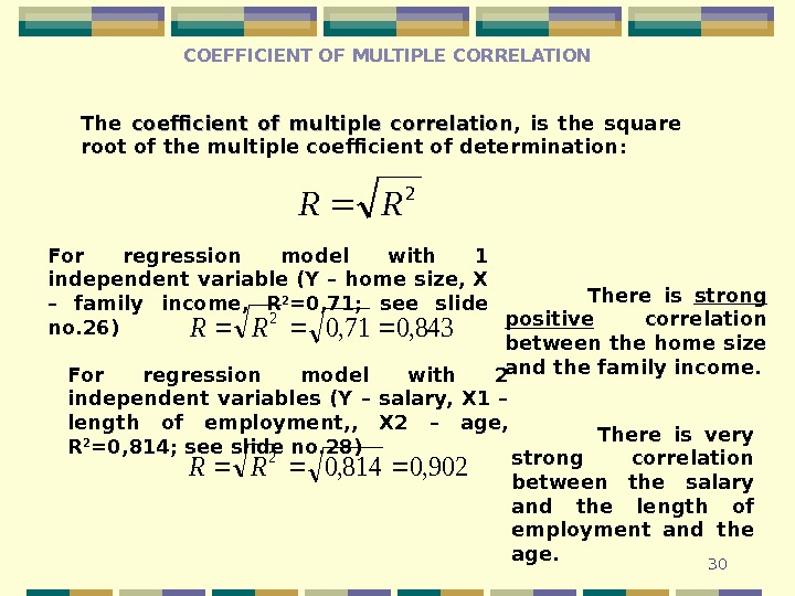
30 COEFFICIENT OF MULTIPLE CORRELATION 2 RR The coefficient of multiple correlation , is the square root of the multiple coefficient of determination : For regression model with 1 independent variable (Y – home size, X – family income, R 2 =0, 71; see slide no. 26)843, 071, 0 2 RR For regression model with 2 independent variables (Y – salary, X 1 – length of employment, , X 2 – age, R 2 =0, 814; see slide no. 28) 902, 0814, 0 2 RR There is strong positive correlation between the home size and the family income. There is very strong correlation between the salary and the length of employment and the age.