6776e9191e8ee6ea6ef4eb251687ea8d.ppt
- Количество слайдов: 25

GLOBAL CHALLENGES and DATA-DRIVEN SCIENCE 8 -13 OCTOBER 2017 SAINT PETERSBURG, RUSSIA Session ID 9 DATA DRIVEN KNOWLEDGE-BASED SYSTEMS FOR BASIC AND APPLIED SCIENCES: COMBUSTION, DETONATION, NANOTECHNOLOGY, RENEWABLE ENERGETICS, ETC Poly. Analyst Data Mining Algorithms for propellants combustion research The reported study was funded by the Russian Foundation of Basic Researches (RFBR) according to the research project No. 16 -53 -48010. PRESENTED BY: Victor Abrukov and Mikhail Kiselev, Chuvash State University 3/19/2018 1
Two kinds of data mining problems • Prognosis • Description Different tasks – different methods
Prediction • We need to predict value of some parameter, variable characterizing some object property etc. (we call it target variable) knowing other parameters and properties of this object (input variables). To make prediction we use a dataset containing data related to similar objects (or to the same object in the past) where values of input variables and target variable are known. Poly. Analyst analyzes this dataset and builds predictive model. It may be very complex, but our main goal is to make the most accurate prediction – we may not have a slightest idea how the model works – but it does not matter - if it works correctly. • Examples: • Credit scoring. Bank gave credits to many customers in the past. The customers had to provide detailed information about them. Some of them had problems with paying the credit. Using these historical data, bank wishes to create predictive model evaluating that the customer will return the credit without problems. • Prognosis of sales of different brands in retail. A retailer wants to predict demand for different brands or product groups to order the respective amount from suppliers. This prediction is made on the basis of historical data where sale volume demonstrated its dependence on time of year, brand novelty, presence of similar products, marketing actions and many other factors. • Automated redirection of customer letters to the appropriate CRM specialist. A corporation has a great set of customer requests manually distributed to the correct staff member responsible to reply to the given request type. This manually classified text corpus is used to create a classifying model which selects the most relevant addressee of the new customer request on the basis of its content.
Description • We would like to understand which factors and in which combination determine value of target variable. Again, a dataset containing known values of input and target variables is used but in this case a key point is interpretation of the found model expressing dependency of target variable on input variables. The model can be suboptimal in terms of its accuracy but it should be clear – the analyst should understand how input variables form the value of target variable. • Examples: • Customer loyalty. Service provider needs to know why people go to its competitors – in order to remove these negative factors and increase customer satisfaction. It solves this problem using its historical data and creating classifying model distinguishing loyal and non-loyal clients. Interpreting this model, company analysts can deduce what are the main causes of customer dissatisfaction. • Drugs adversary side effects. Even very reliable drugs may cause under certain conditions unexpected side effects. Drug manufacturers accumulate descriptions of these undesirable cases. Poly. Analysts creates a classification model separating these exceptional cases from normal drug usage. This model can be used to make a conclusion in which cases the given drug should not be prescribed. • Client satisfaction analysis. Hotel network asks its clients to give evaluation of the service quality. The questionary contains formal data (age, gender etc. ) as well as free edit text field. Using these data the hotels owner creates model predicting customer satisfaction from customer personal data and content of his/her feedback. This model contains valuable information summarizing which kind of customers are not satisfied and what are the main problems of this hotel network or/and of some concrete hotels.

SECTION 1. PREDICTION
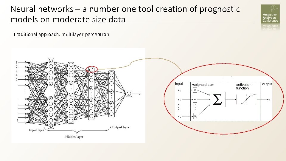
Neural networks – a number one tool creation of prognostic models on moderate size data Traditional approach: multilayer perceptron
Multilayer perceptron • Due to interaction between inputs and non-linear activation function multilayer perceptron can approximate (theoretically) any multidimensional non-linear function. • More layers -> more capabilities to approximate complex functions. • The crucial question – appropriate selection of synaptic weights (learning). • The most frequent approach – error backpropagation algorithm.
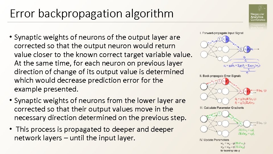
Error backpropagation algorithm • Synaptic weights of neurons of the output layer are corrected so that the output neuron would return value closer to the known correct target variable value. At the same time, for each neuron on previous layer direction of change of its output value is determined which would decrease prediction error for the example presented. • Synaptic weights of neurons from the lower layer are corrected so that their output values move in the necessary direction determined on the previous step. • This process is propagated to deeper and deeper network layers – until the input layer.
Two problems of big perceptrons • In order to make exact predictions in cases when target variable depends on many input variables in complex and non-linear combinations the perceptron should be big – should include many neurons and many layers. However, learning of the big perceptrons faces two fundamental problems: • Over-fitting. Big perceptrons have many synaptic weights. If to consider big perceptron as a regression model, this model would have many degrees of freedom. Using these degrees of freedom the model can fit all statistical fluctuations in training data and approximate target variable with great accuracy, but it will give wrong predictions on new data. It is problematic to choose an appropriate number of degrees of freedom. • Slow and unstable learning. If the perceptron has many layers, it is very difficult to “propagate” error to its deep layers (the deep learning problem). Going from upper level to deeper levels, the link between variation of weight and prediction error becomes weaker and weaker. Variation of an individual weight on a deep layer has almost no impact on output value of the whole perceptron. So that there is great risk to move in a wrong direction.
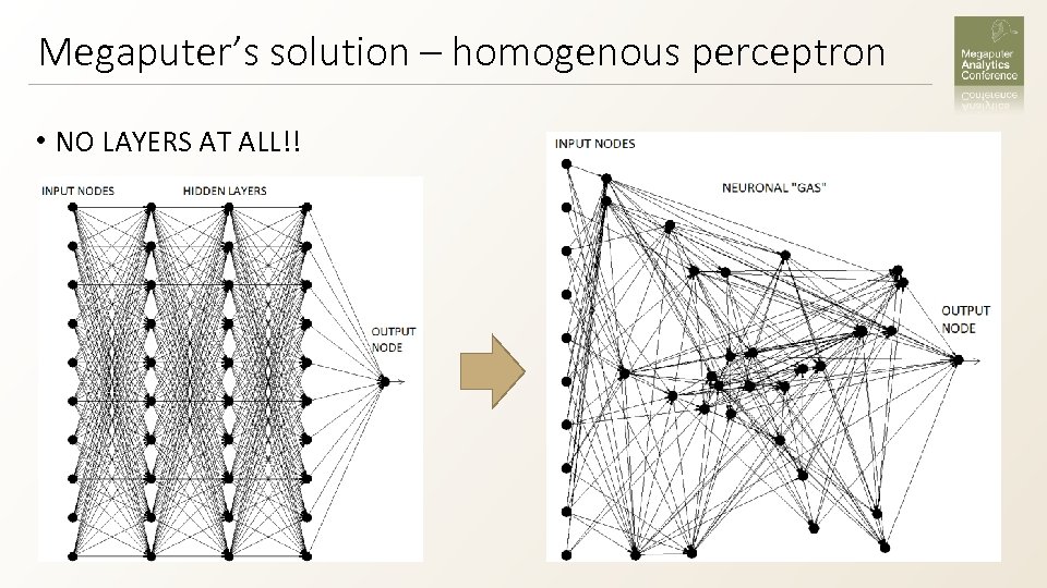
Megaputer’s solution – homogenous perceptron • NO LAYERS AT ALL!!
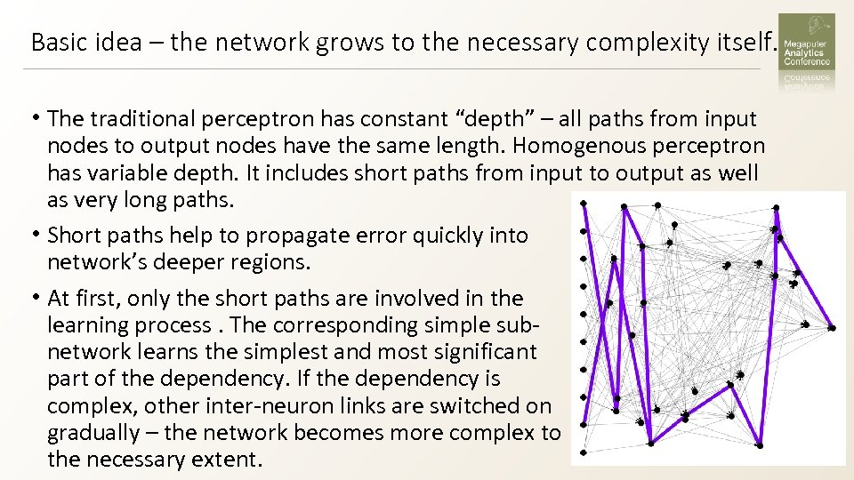
Basic idea – the network grows to the necessary complexity itself. • The traditional perceptron has constant “depth” – all paths from input nodes to output nodes have the same length. Homogenous perceptron has variable depth. It includes short paths from input to output as well as very long paths. • Short paths help to propagate error quickly into network’s deeper regions. • At first, only the short paths are involved in the learning process. The corresponding simple subnetwork learns the simplest and most significant part of the dependency. If the dependency is complex, other inter-neuron links are switched on gradually – the network becomes more complex to the necessary extent.
Homogenous perceptron is a very powerful tool – but… It performs bad in two important cases: • Big data. Training of big neural networks of any kind is a complex process. It includes many cycles (epochs) of weight recalculation for every presented data record. If there are very many records, this process requires unacceptably long time. It is why neural networks are rarely used for analysis of big data. • Small data, wide table. It is not seldom in practical applications that the problem is just the opposite – training examples are few (several hundreds or even tens), but every example is described by many variables (hundreds, thousands…). In this case, risk is overfitting becomes very high. Neural networks have no reliable mechanisms to prevent overfitting in such extreme tasks.
Possible solutions for Big Data • Sampling. It is a simple solution but in many cases it appears to be very efficient. If the dependency of target variable on input variable is simple, then the whole huge dataset is not necessary to discover it. It is sufficient to prepare its small random sample and train network on it. Using the whole dataset would imply only great computation time – but not greater accuracy. • Using fast data mining algorithms. • Probably the fastest method is Naïve Bayes Classifier. It is not very accurate but is very fast – it is a one-pass algorithms involving simple computations. • A slower method (but much more accurate) is Adaptive Boosting. It build an ensemble of tree-like classifiers such that any new added tree classifier concentrates on the records where existing trees gave wrong answers. Creation of each tree is comparatively simple procedure with computation time linearly depending on number of records. • Two above mentioned algorithms solve classification problems. If target variable is numeric, then multiple linear regression with automated predictor selection could be a good solution. In fact, due to implicit non-linear interdependencies between input variables, it can approximate non-linear dependencies as well.
A solution for small wide tables • Random Forest. It is a set of tree-like classifiers. These classifiers can be considered as almost independent because they are built on different subsets of input variables. Classifying a new example, they vote for their decision. Majority wins. This method works because of an interesting statistical trick. When examples are too few to make a statistically significant decision the necessary statistics is obtained using big ensemble of independent classifiers applied to the same example. It may seem like a kind of cheating, but it works!

Other algorithms • Support Vector Machine. This method tries to find a hyperplane in the space of input variable values which would separate records belonging to the different classes. Since only few points are necessary to determine the separating plane, SVM can be used in case of wide tables Moreover, if it is impossible to find a separating hyperplane, the space dimensionality is artificially increased – and it becomes possible!
Other algorithms • Case Based Reasoning. In some cases the best solution is obtained using the following very simple method. If value of target variable should be predicted for a new record, similar records (neighbors) with known target values are found and the prediction is made on the basis of these existing records. This procedure contains three unknowns: what is “similar”, what number of the similar records should be used, and how to calculate prediction from the known target values. The optimum values of these algorithm parameters (record proximity measure, size of neighborhood, and weighted/unweighted averaging procedure) are determined using an appropriate optimization technique, for example, genetic algorithm. Poly. Analyst offers large set of data analysis tools. Often the best tool for the given task is determined using trials and errors.

SECTION 2. DESCRIPTION
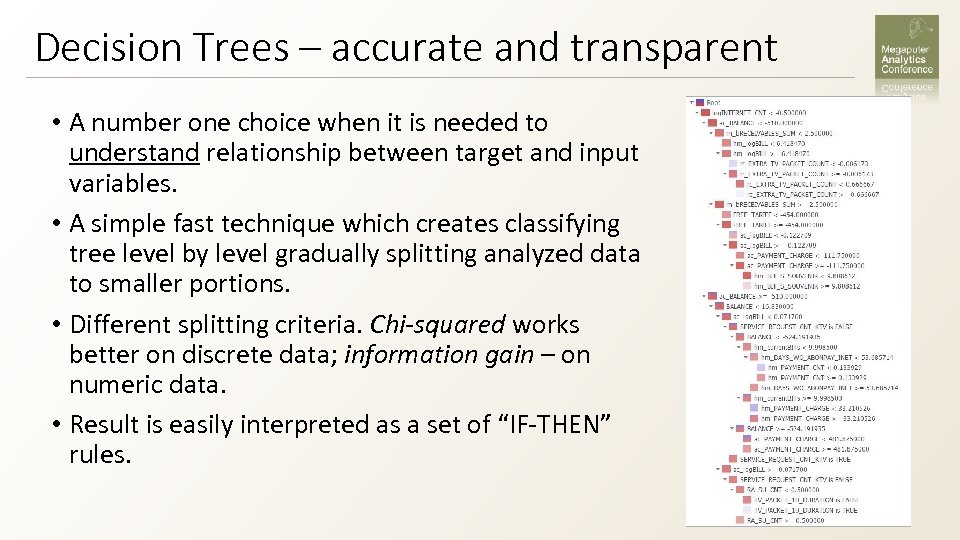
Decision Trees – accurate and transparent • A number one choice when it is needed to understand relationship between target and input variables. • A simple fast technique which creates classifying tree level by level gradually splitting analyzed data to smaller portions. • Different splitting criteria. Chi-squared works better on discrete data; information gain – on numeric data. • Result is easily interpreted as a set of “IF-THEN” rules.
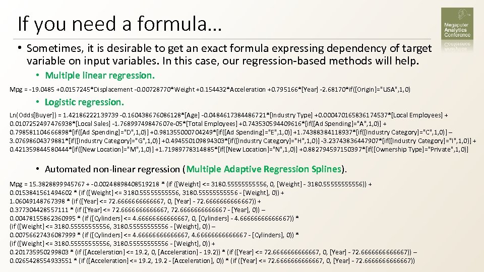
If you need a formula… • Sometimes, it is desirable to get an exact formula expressing dependency of target variable on input variables. In this case, our regression-based methods will help. • Multiple linear regression. Mpg = -19. 0485 +0. 0157245*Displacement -0. 00728770*Weight +0. 154432*Acceleration +0. 795166*[Year] -2. 68170*if([Origin]="USA", 1, 0) • Logistic regression. Ln(Odds[Buyer]) = 1. 42186222139739 -0. 160438676086128*[Age] -0. 0484617384486721*[Industry Type] +0. 000470165836174537*[Local Employees] + 0. 0107252497476938*[Local Sales] -1. 76899749847607 e-05*[Total Employees] +0. 743530594409616*[if([Ad Spending]="A", 1, 0)] + 0. 798581104666898*[if([Ad Spending]="D", 1, 0)] +0. 981355000704249*[if([Ad Spending]="E", 1, 0)] +1. 74388384118937*[if([Industry Category]="C", 1, 0)] – 3. 07698604379881*[if([Industry Category]="G", 1, 0)] +0. 494550109894303*[if([Industry Category]="H", 1, 0)] -3. 23743836447907*[if([Industry Category]="I", 1, 0)] + 0. 421359844580444*[if([New Location]="M", 1, 0)] +1. 71989778314885*[if([New Location]="N", 1, 0)] +0. 882794597150397*[if([Ownership Type]="Private", 1, 0)] • Automated non-linear regression (Multiple Adaptive Regression Splines). Mpg = 15. 3828899945767 + -0. 00248898408519218 * (if ([Weight] <= 3180. 555556, 0, [Weight] - 3180. 555556)) + 0. 0153841561494602 * (if ([Weight] <= 3180. 555556, 3180. 555556 - [Weight], 0)) + 1. 06049148767398 * (if ([Year] <= 72. 6666667, 0, [Year] - 72. 6666667)) + 0. 377304428557111 * (if ([Year] <= 72. 6666667, 72. 6666667 - [Year], 0)) – 0. 00478155862360995 * (if ([Cylinders] <= 4. 66666667, 0, [Cylinders] - 4. 66666667)) * (if ([Weight] <= 3180. 555556, 3180. 555556 - [Weight], 0)) – 0. 00756627436087999 * (if ([Cylinders] <= 4. 66666667, 4. 66666667 - [Cylinders], 0)) * (if ([Weight] <= 3180. 555556, 3180. 555556 - [Weight], 0)) + 0. 201735950299803 * (if ([Acceleration] <= 19. 2, 0, [Acceleration] - 19. 2)) * (if ([Year] <= 72. 6666667, 0, [Year] - 72. 6666667)) – 0. 0265428554933551 * (if ([Acceleration] <= 19. 2, 19. 2 - [Acceleration], 0)) * (if ([Year] <= 72. 6666667, 0, [Year] - 72. 6666667))
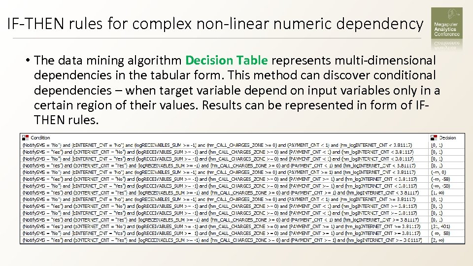
IF-THEN rules for complex non-linear numeric dependency • The data mining algorithm Decision Table represents multi-dimensional dependencies in the tabular form. This method can discover conditional dependencies – when target variable depend on input variables only in a certain region of their values. Results can be represented in form of IFTHEN rules.

SECTION 3. EXAMPLE Prediction of Propellants Burning Rate
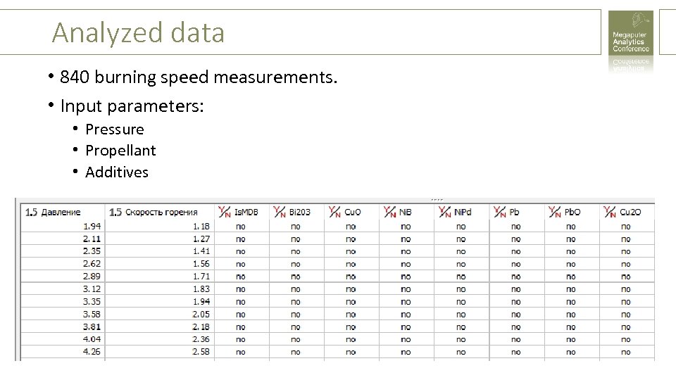
Analyzed data • 840 burning speed measurements. • Input parameters: • Pressure • Propellant • Additives
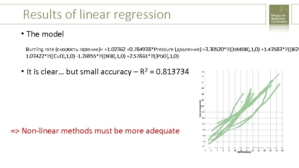
Results of linear regression • The model Burning rate (скорость горения)= +1. 02362 +0. 784938*Pressure (давление) +3. 30520*if([Is. MDB], 1, 0) +1. 43583*if([Bi 20 1. 03422*if([Cu. O], 1, 0) -1. 26955*if([Ni. B], 1, 0) +2. 57861*if([Pb. O], 1, 0) • It is clear… but small accuracy – R 2 = 0. 813734 => Non-linear methods must be more adequate
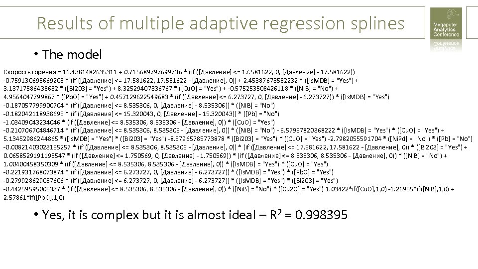
Results of multiple adaptive regression splines • The model Скорость горения = 16. 4381482635311 + 0. 715689797699736 * (if ([Давление] <= 17. 581622, 0, [Давление] - 17. 581622)) -0. 759130695669203 * (if ([Давление] <= 17. 581622, 17. 581622 - [Давление], 0)) + 2. 45387673582232 * ([Is. MDB] = "Yes") + 3. 13717586438632 * ([Bi 203] = "Yes") + 8. 32529407336767 * ([Cu. O] = "Yes") + -0. 575253508426118 * ([Ni. B] = "No") + 4. 9564047799867 * ([Pb. O] = "Yes") + 0. 457129622549683 * (if ([Давление] <= 6. 273727, 0, [Давление] - 6. 273727)) * ([Is. MDB] = "Yes") -0. 187057799900704 * (if ([Давление] <= 8. 535306, 0, [Давление] - 8. 535306)) * ([Ni. B] = "No") -0. 182042118938695 * (if ([Давление] <= 15. 320043, 0, [Давление] - 15. 320043)) * ([Pb] = "No") -1. 03409043234046 * (if ([Давление] <= 8. 535306, 8. 535306 - [Давление], 0)) * ([Cu. O] = "Yes") -0. 210706704846714 * (if ([Давление] <= 8. 535306, 8. 535306 - [Давление], 0)) * ([Ni. B] = "No") - 6. 57957820368222 * ([Is. MDB] = "Yes") * ([Cu. O] = "Yes") + 5. 13452986244865 * ([Is. MDB] = "Yes") * ([Bi 203] = "Yes") -8. 57965785773878 * ([Bi 203] = "Yes") * ([Cu. O] = "Yes") -2. 7982055591704 * ([Ni. Pd] = "No") * ([Pb] = "No") -0. 00821403023155257 * (if ([Давление] <= 8. 535306, 8. 535306 - [Давление], 0)) * (if ([Давление] <= 17. 581622, 17. 581622 - [Давление], 0)) * ([Bi 203] = "Yes") + 0. 0658529191195547 * (if ([Давление] <= 1. 750569, 0, [Давление] - 1. 750569)) * (if ([Давление] <= 8. 535306, 8. 535306 - [Давление], 0)) * ([Ni. B] = "No") + 1. 00400458350309 * (if ([Давление] <= 8. 535306, 8. 535306 - [Давление], 0)) * ([Is. MDB] = "Yes") * ([Cu. O] = "Yes") -0. 221931768073874 * (if ([Давление] <= 6. 273727, 0, [Давление] - 6. 273727)) * ([Is. MDB] = "Yes") * ([Pb. O] = "Yes") -0. 279928629057606 * (if ([Давление] <= 6. 273727, 0, [Давление] - 6. 273727)) * ([Is. MDB] = "Yes") * ([Bi 203] = "Yes") -0. 44259595005337 * (if ([Давление] <= 8. 535306, 8. 535306 - [Давление], 0)) * ([Ni. B] = "No") * ([Cu 2 O] = "Yes") 1. 03422*if([Cu. O], 1, 0) -1. 26955*if([Ni. B], 1, 0) + 2. 57861*if([Pb. O], 1, 0) • Yes, it is complex but it is almost ideal – R 2 = 0. 998395
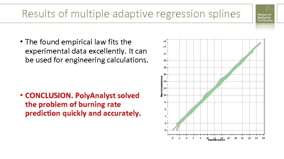
Results of multiple adaptive regression splines • The found empirical law fits the experimental data excellently. It can be used for engineering calculations. • CONCLUSION. Poly. Analyst solved the problem of burning rate prediction quickly and accurately.
6776e9191e8ee6ea6ef4eb251687ea8d.ppt