GIS Analysis Concepts Copyright C Schweik M Fernandez 2007

GIS Analysis Concepts Copyright C. Schweik/M. Fernandez 2007 (Some material adapted from Heywood et al 1998; Theobald, 1999 ) 1

What kinds of analysis can we do with GIS? 1. Measurements 2. Layer statistics 3. Queries 4. Buffering (vector); Proximity (raster) 5. Filtering (raster) 6. Map overlay (layer on layer selections) 7. Transformations 8. Reclassification 9. Network analysis 10. Spatial interpolation 11. Grid (raster) analysis 12. Surface analysis 13. Analytic modeling 2

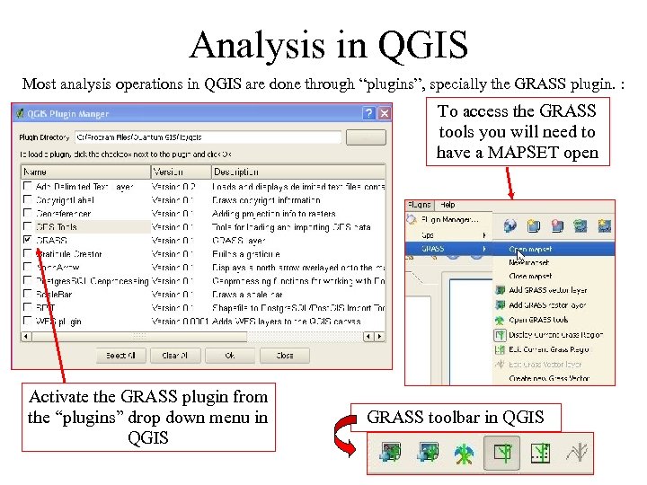Analysis in QGIS Most analysis operations in QGIS are done through “plugins”, specially the GRASS plugin. : To access the GRASS tools you will need to have a MAPSET open Activate the GRASS plugin from the “plugins” drop down menu in QGIS GRASS toolbar in QGIS

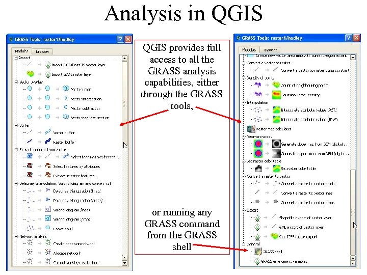Analysis in QGIS provides full access to all the GRASS analysis capabilities, either through the GRASS tools, or running any GRASS command from the GRASS shell

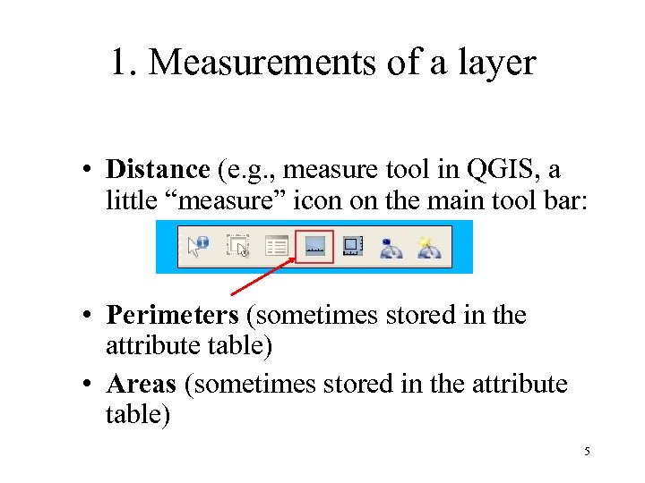1. Measurements of a layer • Distance (e. g. , measure tool in QGIS, a little “measure” icon on the main tool bar: • Perimeters (sometimes stored in the attribute table) • Areas (sometimes stored in the attribute table) 5

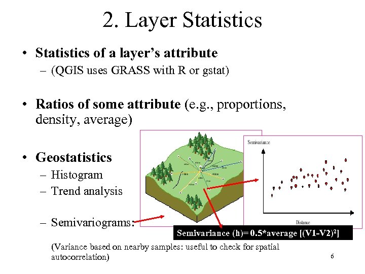2. Layer Statistics • Statistics of a layer’s attribute – (QGIS uses GRASS with R or gstat) • Ratios of some attribute (e. g. , proportions, density, average) • Geostatistics – Histogram – Trend analysis – Semivariograms: Semivariance (h)= 0. 5*average [(V 1 -V 2)2] (Variance based on nearby samples: useful to check for spatial autocorrelation) 6

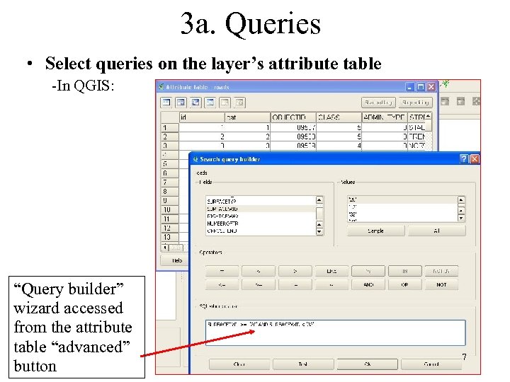3 a. Queries • Select queries on the layer’s attribute table -In QGIS: “Query builder” wizard accessed from the attribute table “advanced” button 7

3 b. Queries • Neighborhood analysis queries: –What’s adjacent? –What’s nearby? (In QGIS done with “buffer” and “intersection” operations, explained later in this presentation) • Sampling -Select (randomly or not) a subset of features and create a new layer based on them.

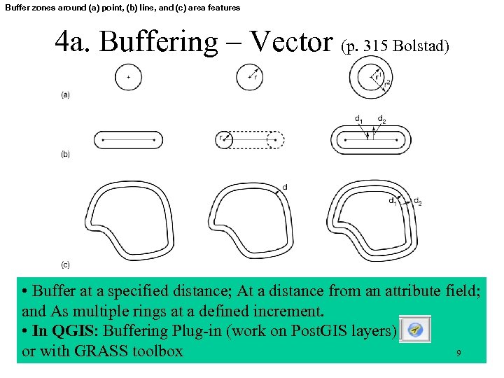Buffer zones around (a) point, (b) line, and (c) area features 4 a. Buffering – Vector (p. 315 Bolstad) • Buffer at a specified distance; At a distance from an attribute field; and As multiple rings at a defined increment. • In QGIS: Buffering Plug-in (work on Post. GIS layers) 9 or with GRASS toolbox

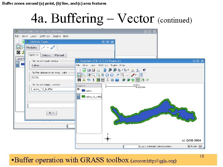Buffer zones around (a) point, (b) line, and (c) area features 4 a. Buffering – Vector (continued) • Buffer operation with GRASS toolbox (source: http: //qgis. org) 10

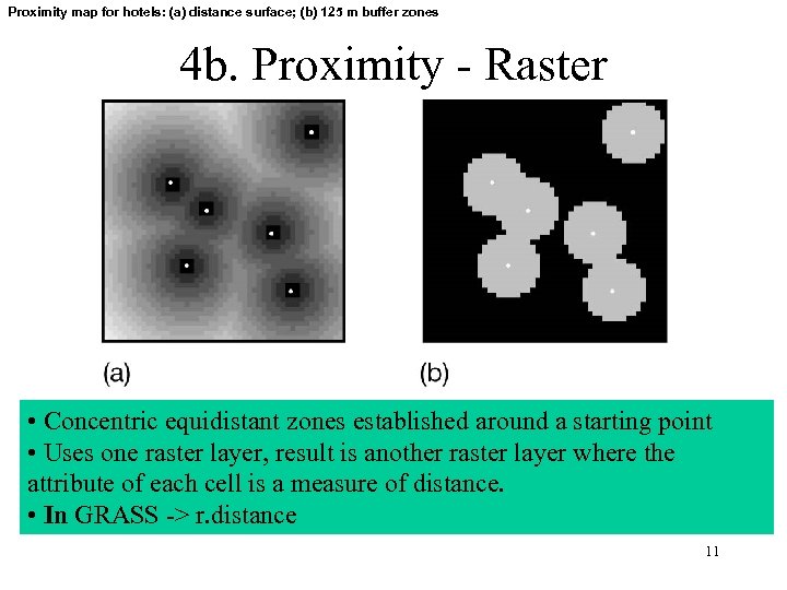Proximity map for hotels: (a) distance surface; (b) 125 m buffer zones 4 b. Proximity - Raster • Concentric equidistant zones established around a starting point • Uses one raster layer, result is another raster layer where the attribute of each cell is a measure of distance. • In GRASS -> r. distance 11

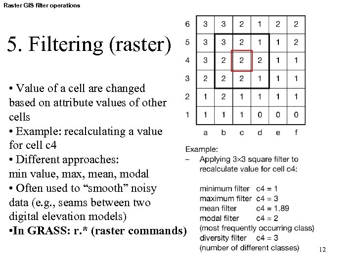Raster GIS filter operations 5. Filtering (raster) • Value of a cell are changed based on attribute values of other cells • Example: recalculating a value for cell c 4 • Different approaches: min value, max, mean, modal • Often used to “smooth” noisy data (e. g. , seams between two digital elevation models) • In GRASS: r. * (raster commands) 12

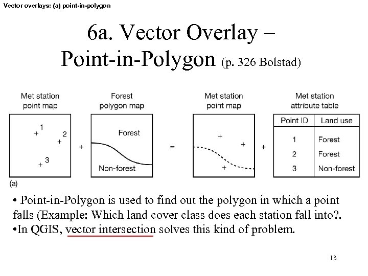Vector overlays: (a) point-in-polygon 6 a. Vector Overlay – Point-in-Polygon (p. 326 Bolstad) • Point-in-Polygon is used to find out the polygon in which a point falls (Example: Which land cover class does each station fall into? . • In QGIS, vector intersection solves this kind of problem. 13

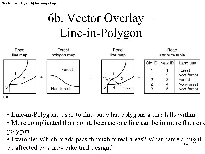Vector overlays: (b) line-in-polygon 6 b. Vector Overlay – Line-in-Polygon • Line-in-Polygon: Used to find out what polygons a line falls within. • More complicated than point, because one line can be in more than one polygon • Example: Which roads pass through forest areas? What parcels might 14 be affected by a new bike trail design?

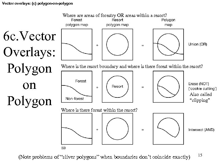Vector overlays: (c) polygon-on-polygon Where areas of forestry OR areas within a resort? 6 c. Vector Overlays: Polygon on Polygon Where is the resort boundary and where is there forest within the resort? Also called “clipping” Where is there forest within the resort? (Note problems of “sliver polygons” when boundaries don’t coincide exactly) 15

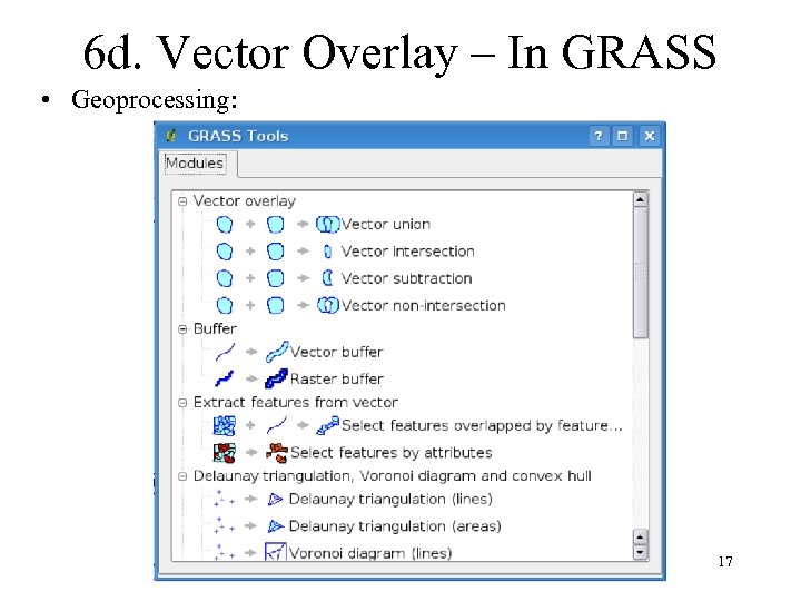6 d. Vector Overlay – In GRASS • Geoprocessing: 17

6 e. Raster Overlay • “Map Algebra” or “Mapematics” • Two raster layers with same cell size • Can add, subtract, multiply, divide them to produce a new layer • In QGIS: GRASS Tools: “Raster Map Calculator”: r. mapcalc or any raster operation from the GRASS shell. [see: http: //grass. itc. it/grass 61/manuals/html 61_user/rasterintro. html] 18

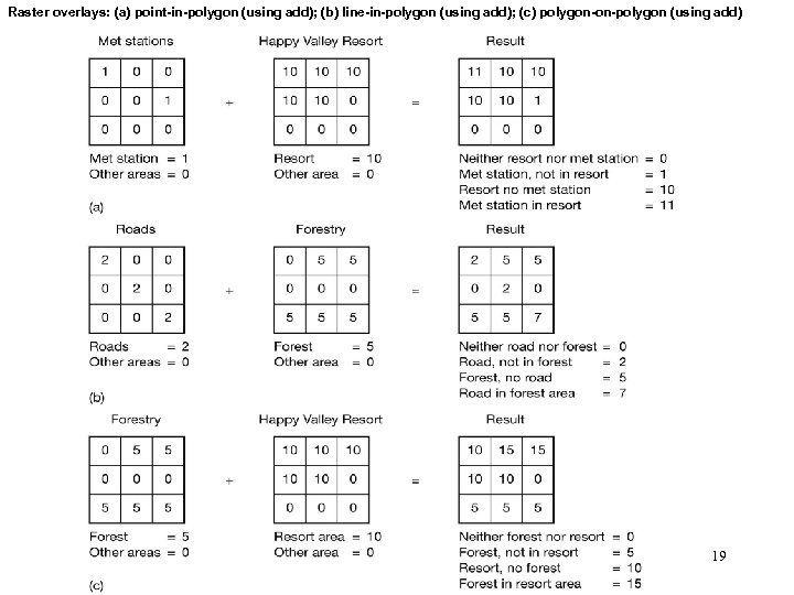Raster overlays: (a) point-in-polygon (using add); (b) line-in-polygon (using add); (c) polygon-on-polygon (using add) 19

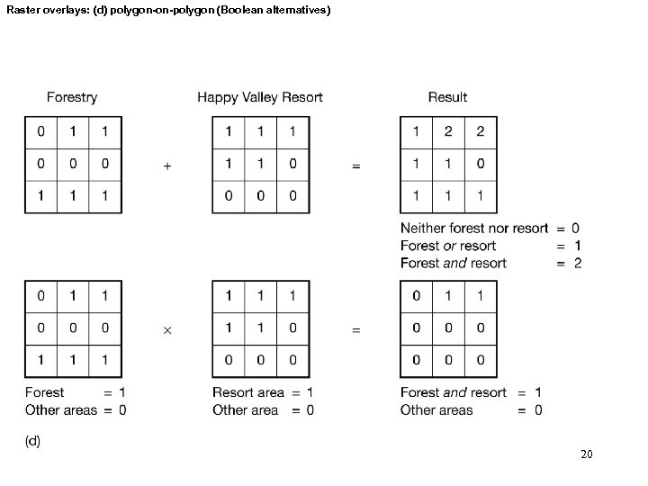Raster overlays: (d) polygon-on-polygon (Boolean alternatives) 20

7. Transformations • Functions to transform a layer of one feature type to another. Some examples: – Point to line: interpolation (contour mapping) – Point to polygon: buffering – Polygon to polygon: dissolve/merge • • Raster to vector conversion Vector to raster conversion Raster to Triangular Irregular Network (TIN) Resampling a raster grid – convert one cell size to another cell size 21

8. Reclassification • Converting attribute table field values to some new field and values • Example: Converting a landuse layer with 21 different landuse categories to a layer that is just “forest (1) or no forest (0). ” Polygons with value of 10 (forest) should get a value of 1 (yes); otherwise 0 (no). – Example: Satellite image classification • Can be done in vector or raster 22

9. Network Analysis • Networks are sets of interconnected lines through which resources can flow. – E. g. , roads, rivers, powerlines – Concept of “Impedance values” (attributes of line segments such as speed limits of roads, etc) • Classic networking problems: – Shortest path – Traveling salesman problem (visit many locations in a day – what is the quickest route to them all? ) – Location-Allocation modeling (e. g. , matching supply of services with demand through a road network) – Route tracing (ability to trace the flow of goods, people, services or information through a network of lines) 23

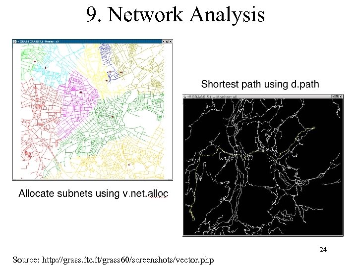9. Network Analysis 24 Source: http: //grass. itc. it/grass 60/screenshots/vector. php

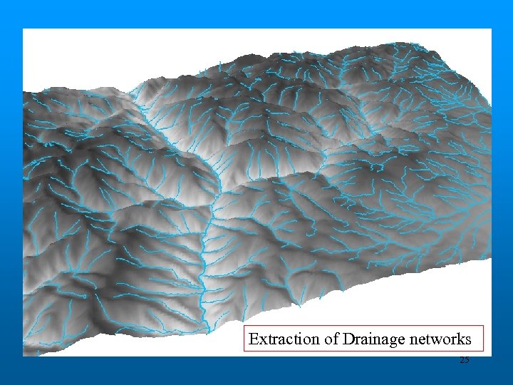Extraction of Drainage networks 25

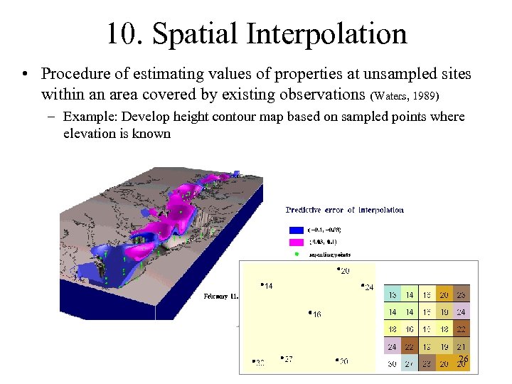10. Spatial Interpolation • Procedure of estimating values of properties at unsampled sites within an area covered by existing observations (Waters, 1989) – Example: Develop height contour map based on sampled points where elevation is known 26

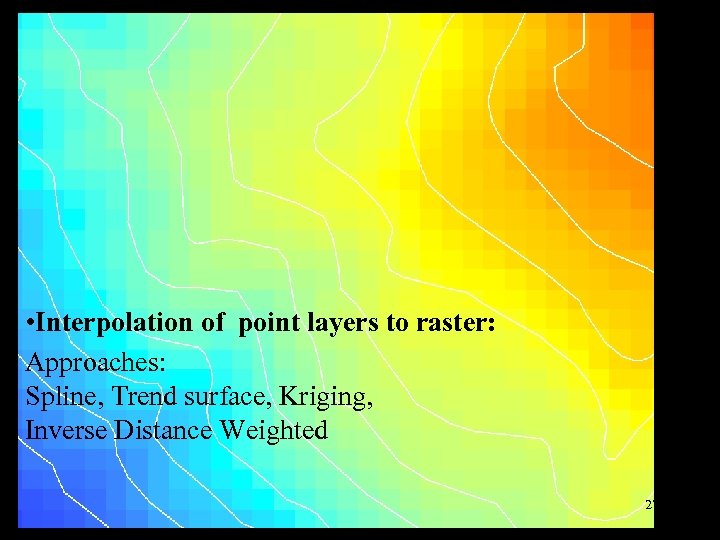• Interpolation of point layers to raster: Approaches: Spline, Trend surface, Kriging, Inverse Distance Weighted 27

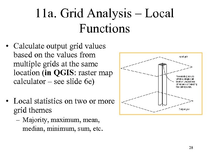11 a. Grid Analysis – Local Functions • Calculate output grid values based on the values from multiple grids at the same location (in QGIS: raster map calculator – see slide 6 e) • Local statistics on two or more grid themes – Majority, maximum, mean, median, minimum, sum, etc. 28

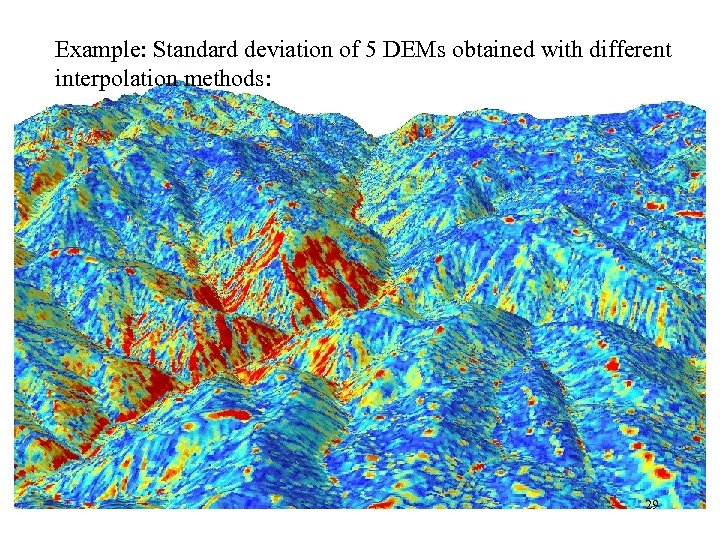Example: Standard deviation of 5 DEMs obtained with different interpolation methods: 29

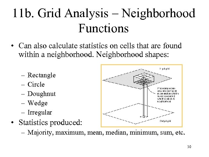11 b. Grid Analysis – Neighborhood Functions • Can also calculate statistics on cells that are found within a neighborhood. Neighborhood shapes: – – – Rectangle Circle Doughnut Wedge Irregular • Statistics produced: – Majority, maximum, mean, median, minimum, sum, etc. 30

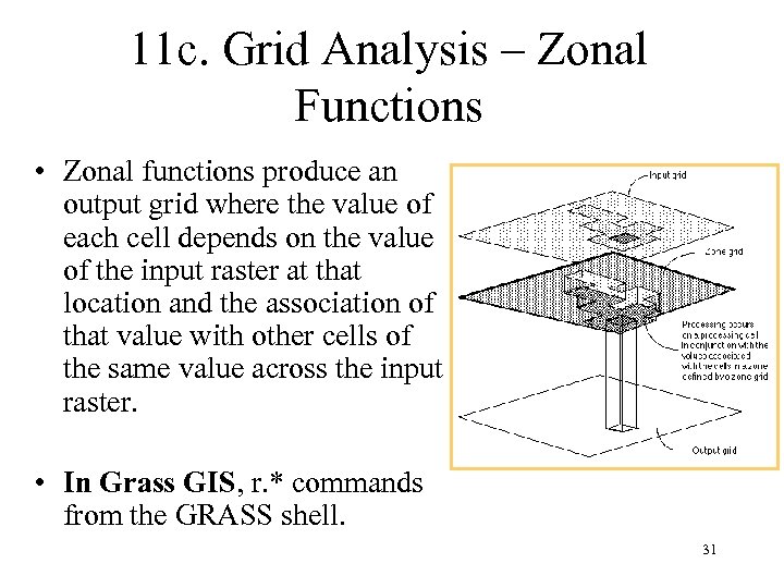11 c. Grid Analysis – Zonal Functions • Zonal functions produce an output grid where the value of each cell depends on the value of the input raster at that location and the association of that value with other cells of the same value across the input raster. • In Grass GIS, r. * commands from the GRASS shell. 31

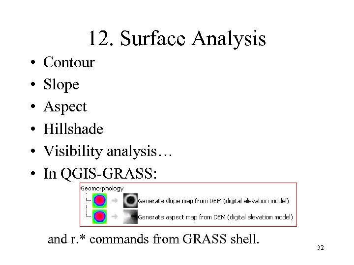12. Surface Analysis • • • Contour Slope Aspect Hillshade Visibility analysis… In QGIS-GRASS: and r. * commands from GRASS shell. 32

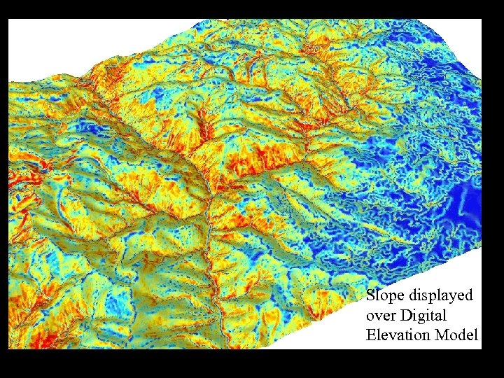Slope displayed over Digital Elevation Model 33