Genetic design Testing Mendelian segregation Consider marker

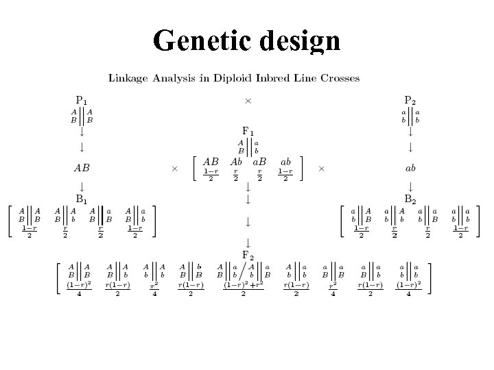Genetic design

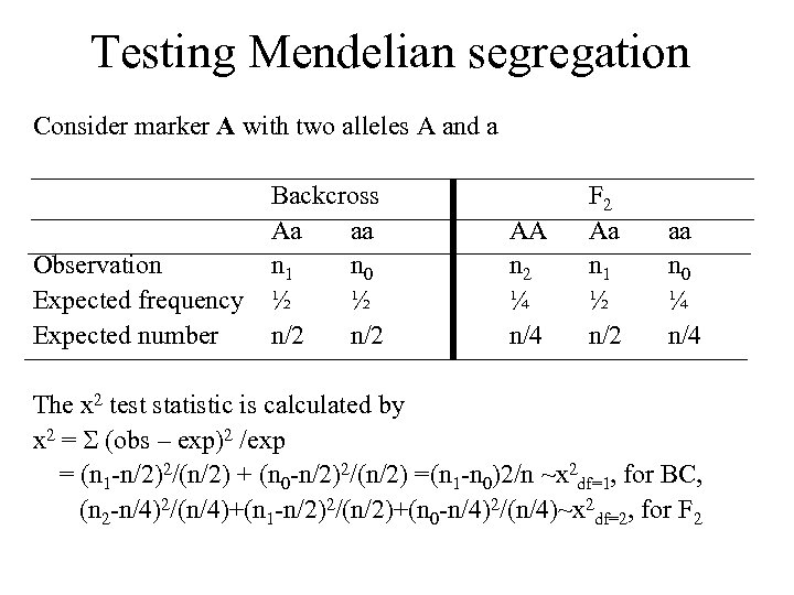Testing Mendelian segregation Consider marker A with two alleles A and a Observation Expected frequency Expected number Backcross Aa aa n 1 n 0 ½ ½ n/2 AA n 2 ¼ n/4 F 2 Aa n 1 ½ n/2 aa n 0 ¼ n/4 The x 2 test statistic is calculated by x 2 = (obs – exp)2 /exp = (n 1 -n/2)2/(n/2) + (n 0 -n/2)2/(n/2) =(n 1 -n 0)2/n ~x 2 df=1, for BC, (n 2 -n/4)2/(n/4)+(n 1 -n/2)2/(n/2)+(n 0 -n/4)2/(n/4)~x 2 df=2, for F 2

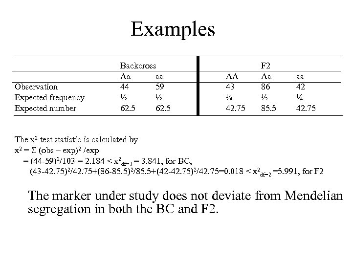Examples Observation Expected frequency Expected number Backcross Aa aa 44 59 ½ ½ 62. 5 AA 43 ¼ 42. 75 F 2 Aa 86 ½ 85. 5 aa 42 ¼ 42. 75 The x 2 test statistic is calculated by x 2 = (obs – exp)2 /exp = (44 -59)2/103 = 2. 184 < x 2 df=1 = 3. 841, for BC, (43 -42. 75)2/42. 75+(86 -85. 5)2/85. 5+(42 -42. 75)2/42. 75=0. 018 < x 2 df=2 =5. 991, for F 2 The marker under study does not deviate from Mendelian segregation in both the BC and F 2.

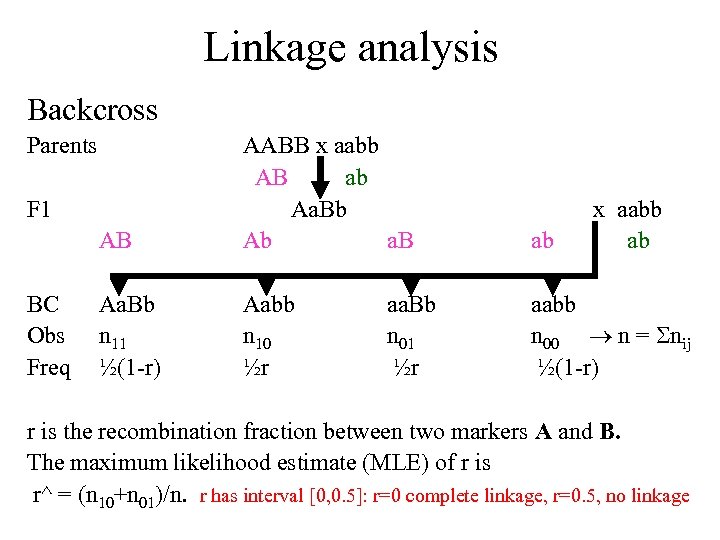Linkage analysis Backcross Parents AB AABB x aabb AB ab Aa. Bb Ab a. B ab Aa. Bb n 11 ½(1 -r) Aabb n 10 ½r aabb n 00 n = nij ½(1 -r) F 1 BC Obs Freq aa. Bb n 01 ½r x aabb ab r is the recombination fraction between two markers A and B. The maximum likelihood estimate (MLE) of r is r^ = (n 10+n 01)/n. r has interval [0, 0. 5]: r=0 complete linkage, r=0. 5, no linkage

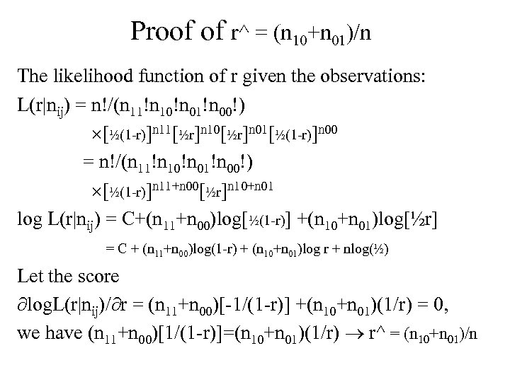Proof of r^ = (n 10+n 01)/n The likelihood function of r given the observations: L(r|nij) = n!/(n 11!n 10!n 01!n 00!) [½(1 -r)]n 11[½r]n 10[½r]n 01[½(1 -r)]n 00 = n!/(n 11!n 10!n 01!n 00!) [½(1 -r)]n 11+n 00[½r]n 10+n 01 log L(r|nij) = C+(n 11+n 00)log[½(1 -r)] +(n 10+n 01)log[½r] = C + (n 11+n 00)log(1 -r) + (n 10+n 01)log r + nlog(½) Let the score log. L(r|nij)/ r = (n 11+n 00)[-1/(1 -r)] +(n 10+n 01)(1/r) = 0, we have (n 11+n 00)[1/(1 -r)]=(n 10+n 01)(1/r) r^ = (n 10+n 01)/n

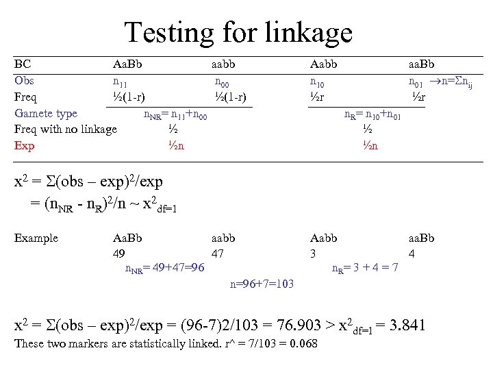Testing for linkage BC Aa. Bb aabb Obs n 11 n 00 Freq ½(1 -r) Gamete type n. NR= n 11+n 00 Freq with no linkage ½ Exp ½n Aabb n 10 ½r aa. Bb n 01 n= nij ½r n. R= n 10+n 01 ½ ½n x 2 = (obs – exp)2/exp = (n. NR - n. R)2/n ~ x 2 df=1 Example Aa. Bb aabb 49 47 n. NR= 49+47=96 n=96+7=103 Aabb aa. Bb 3 4 n. R= 3 + 4 = 7 x 2 = (obs – exp)2/exp = (96 -7)2/103 = 76. 903 > x 2 df=1 = 3. 841 These two markers are statistically linked. r^ = 7/103 = 0. 068

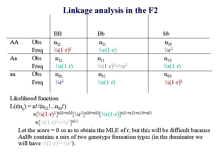Linkage analysis in the F 2 AA Aa aa Obs Freq BB n 22 ¼(1 -r)2 n 12 ½r(1 -r) n 02 ¼r 2 Bb n 21 ½r(1 -r) n 11 ½(1 -r)2+½r 2 n 01 ½r(1 -r) bb n 20 ¼r 2 n 10 ½r(1 -r) n 00 ¼(1 -r)2 Likelihood function L(r|nij) = n!/(n 22!. . . n 00!) [¼(1 -r)2]n 22+n 00[¼r 2]n 20+n 02[½r(1 -r)]n 21+n 12+n 10+n 01 [½(1 -r)2+½r 2]n 11 Let the score = 0 so as to obtain the MLE of r, but this will be difficult because Aa. Bb contains a mix of two genotype formation types (in the dominator we will have ½(1 -r)2+½r 2).

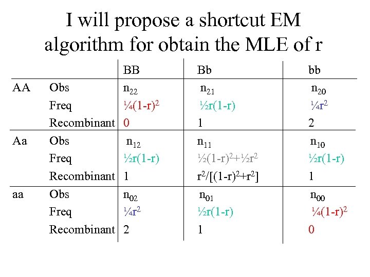I will propose a shortcut EM algorithm for obtain the MLE of r AA Aa aa BB Obs n 22 Freq ¼(1 -r)2 Recombinant 0 Obs n 12 Freq ½r(1 -r) Recombinant 1 Obs n 02 Freq ¼r 2 Recombinant 2 Bb n 21 ½r(1 -r) 1 n 11 ½(1 -r)2+½r 2 r 2/[(1 -r)2+r 2] n 01 ½r(1 -r) 1 bb n 20 ¼r 2 2 n 10 ½r(1 -r) 1 n 00 ¼(1 -r)2 0

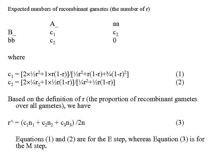
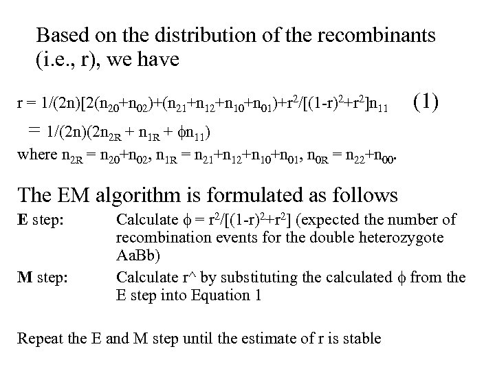Based on the distribution of the recombinants (i. e. , r), we have r = 1/(2 n)[2(n 20+n 02)+(n 21+n 12+n 10+n 01)+r 2/[(1 -r)2+r 2]n 11 (1) = 1/(2 n)(2 n 2 R + n 11) where n 2 R = n 20+n 02, n 1 R = n 21+n 12+n 10+n 01, n 0 R = n 22+n 00. The EM algorithm is formulated as follows E step: M step: Calculate = r 2/[(1 -r)2+r 2] (expected the number of recombination events for the double heterozygote Aa. Bb) Calculate r^ by substituting the calculated from the E step into Equation 1 Repeat the E and M step until the estimate of r is stable

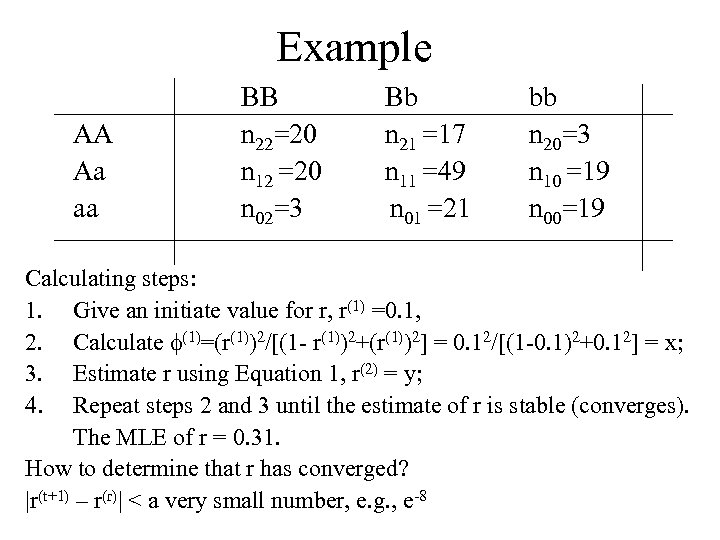Example AA Aa aa BB n 22=20 n 12 =20 n 02=3 Bb n 21 =17 n 11 =49 n 01 =21 bb n 20=3 n 10 =19 n 00=19 Calculating steps: 1. Give an initiate value for r, r(1) =0. 1, 2. Calculate (1)=(r(1))2/[(1 - r(1))2+(r(1))2] = 0. 12/[(1 -0. 1)2+0. 12] = x; 3. Estimate r using Equation 1, r(2) = y; 4. Repeat steps 2 and 3 until the estimate of r is stable (converges). The MLE of r = 0. 31. How to determine that r has converged? |r(t+1) – r(r)| < a very small number, e. g. , e-8

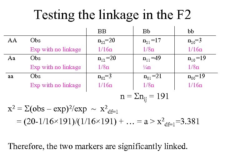Testing the linkage in the F 2 AA Aa aa Obs Exp with no linkage BB n 22=20 1/16 n n 12 =20 1/8 n n 02=3 1/16 n Bb n 21 =17 1/8 n n 11 =49 ¼n n 01 =21 1/8 n bb n 20=3 1/16 n n 10 =19 1/8 n n 00=19 1/16 n n = nij = 191 x 2 = (obs – exp)2/exp ~ x 2 df=1 = (20 -1/16× 191)/(1/16× 191) + … = a > x 2 df=1=3. 381 Therefore, the two markers are significantly linked.

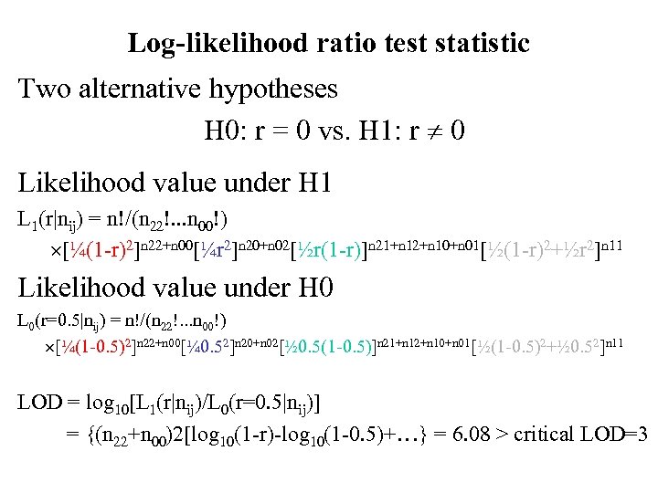Log-likelihood ratio test statistic Two alternative hypotheses H 0: r = 0 vs. H 1: r 0 Likelihood value under H 1 L 1(r|nij) = n!/(n 22!. . . n 00!) [¼(1 -r)2]n 22+n 00[¼r 2]n 20+n 02[½r(1 -r)]n 21+n 12+n 10+n 01[½(1 -r)2+½r 2]n 11 Likelihood value under H 0 L 0(r=0. 5|nij) = n!/(n 22!. . . n 00!) [¼(1 -0. 5)2]n 22+n 00[¼ 0. 52]n 20+n 02[½ 0. 5(1 -0. 5)]n 21+n 12+n 10+n 01[½(1 -0. 5)2+½ 0. 52]n 11 LOD = log 10[L 1(r|nij)/L 0(r=0. 5|nij)] = {(n 22+n 00)2[log 10(1 -r)-log 10(1 -0. 5)+…} = 6. 08 > critical LOD=3

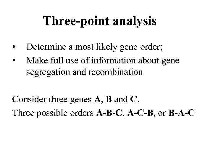Three-point analysis • • Determine a most likely gene order; Make full use of information about gene segregation and recombination Consider three genes A, B and C. Three possible orders A-B-C, A-C-B, or B-A-C

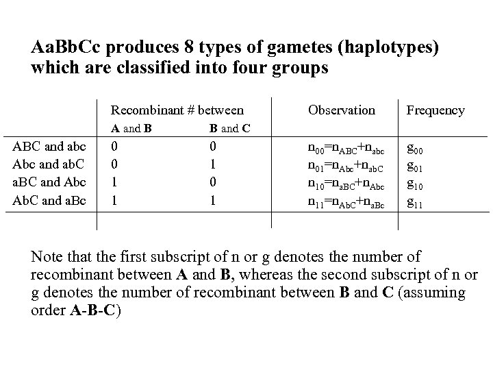Aa. Bb. Cc produces 8 types of gametes (haplotypes) which are classified into four groups Recombinant # between A and B ABC and abc Abc and ab. C a. BC and Abc Ab. C and a. Bc 0 1 Frequency n 00=n. ABC+nabc n 01=n. Abc+nab. C n 10=na. BC+n. Abc n 11=n. Ab. C+na. Bc g 00 g 01 g 10 g 11 B and C 0 0 1 1 Observation Note that the first subscript of n or g denotes the number of recombinant between A and B, whereas the second subscript of n or g denotes the number of recombinant between B and C (assuming order A-B-C)

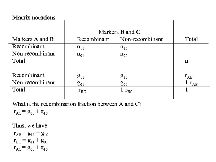Matrix notations Markers A and B Recombinant Non-recombinant Total Markers B and C Recombinant Non-recombinant n 11 n 10 n 01 n 00 g 11 g 01 r. BC g 10 g 00 1 -r. BC What is the recombination fraction between A and C? r. AC = g 01 + g 10 Thus, we have r. AB = g 11 + g 10 r. BC = g 11 + g 01 r. AC = g 01 + g 10 Total n r. AB 1 -r. AB 1

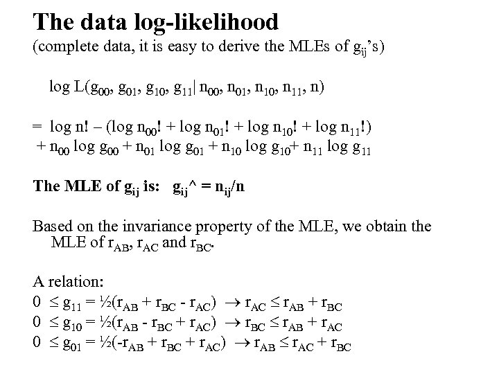The data log-likelihood (complete data, it is easy to derive the MLEs of gij’s) log L(g 00, g 01, g 10, g 11| n 00, n 01, n 10, n 11, n) = log n! – (log n 00! + log n 01! + log n 10! + log n 11!) + n 00 log g 00 + n 01 log g 01 + n 10 log g 10+ n 11 log g 11 The MLE of gij is: gij^ = nij/n Based on the invariance property of the MLE, we obtain the MLE of r. AB, r. AC and r. BC. A relation: 0 g 11 = ½(r. AB + r. BC - r. AC) r. AC r. AB + r. BC 0 g 10 = ½(r. AB - r. BC + r. AC) r. BC r. AB + r. AC 0 g 01 = ½(-r. AB + r. BC + r. AC) r. AB r. AC + r. BC

Advantages of three-point (and generally multi-point) analysis • Determine the gene order, • Increase the estimation precision of the recombination fractions (for partially informative markers).

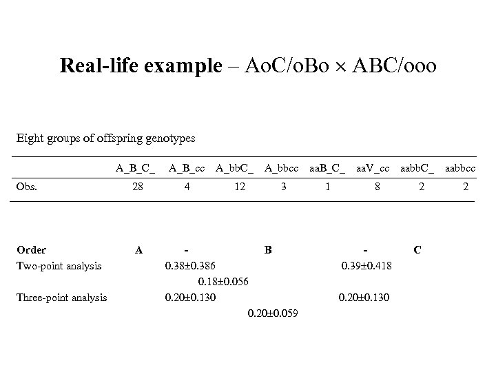Real-life example – Ao. C/o. Bo ABC/ooo Eight groups of offspring genotypes A_B_C_ A_B_cc Obs. 28 4 Order Two-point analysis A Three-point analysis A_bb. C_ 12 A_bbcc aa. B_C_ 3 1 B 0. 386 0. 18 0. 056 0. 20 0. 130 0. 20 0. 059 aa. V_cc 8 0. 39 0. 418 0. 20 0. 130 aabb. C_ 2 C aabbcc 2

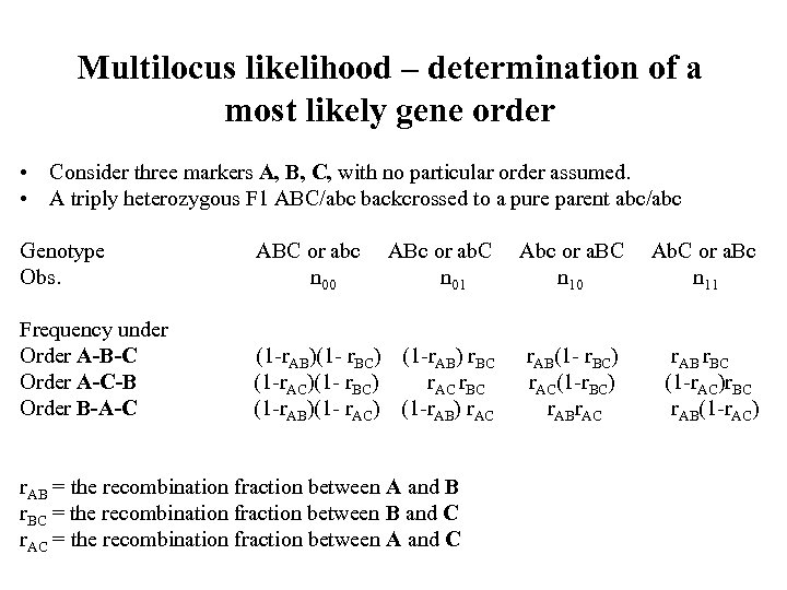Multilocus likelihood – determination of a most likely gene order • Consider three markers A, B, C, with no particular order assumed. • A triply heterozygous F 1 ABC/abc backcrossed to a pure parent abc/abc Genotype Obs. ABC or abc n 00 ABc or ab. C n 01 Abc or a. BC n 10 Ab. C or a. Bc n 11 Frequency under Order A-B-C Order A-C-B Order B-A-C (1 -r. AB)(1 - r. BC) (1 -r. AB) r. BC (1 -r. AC)(1 - r. BC) r. AC r. BC (1 -r. AB)(1 - r. AC) (1 -r. AB) r. AC r. AB(1 - r. BC) r. AC(1 -r. BC) r. ABr. AC r. AB r. BC (1 -r. AC)r. BC r. AB(1 -r. AC) r. AB = the recombination fraction between A and B r. BC = the recombination fraction between B and C r. AC = the recombination fraction between A and C

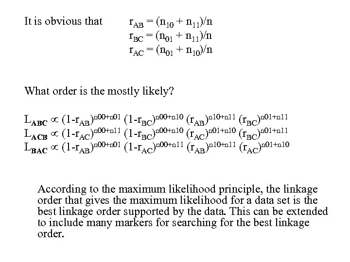It is obvious that r. AB = (n 10 + n 11)/n r. BC = (n 01 + n 11)/n r. AC = (n 01 + n 10)/n What order is the mostly likely? LABC (1 -r. AB)n 00+n 01 (1 -r. BC)n 00+n 10 (r. AB)n 10+n 11 (r. BC)n 01+n 11 LACB (1 -r. AC)n 00+n 11 (1 -r. BC)n 00+n 10 (r. AC)n 01+n 10 (r. BC)n 01+n 11 LBAC (1 -r. AB)n 00+n 01 (1 -r. AC)n 00+n 11 (r. AB)n 10+n 11 (r. AC)n 01+n 10 According to the maximum likelihood principle, the linkage order that gives the maximum likelihood for a data set is the best linkage order supported by the data. This can be extended to include many markers for searching for the best linkage order.

Map function • • Transfer the recombination fraction (non-additivity) between two genes into their corresponding genetic map distance (additivity) Map distance is defined as the mean number of crossovers The unit of map distance is Morgan (in honor of T. H. Morgan who obtained the Novel prize in 1930 s) 1 Morgan or M = 100 centi. Morgan or c. M

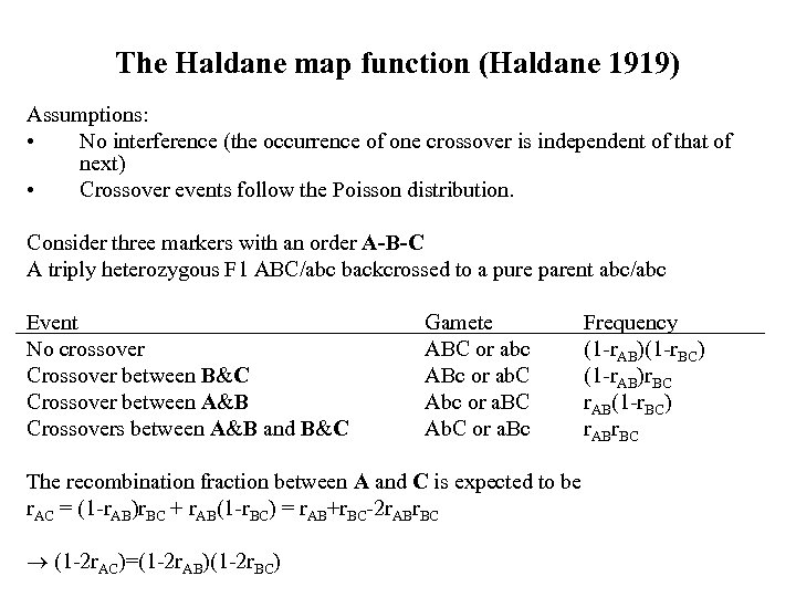The Haldane map function (Haldane 1919) Assumptions: • No interference (the occurrence of one crossover is independent of that of next) • Crossover events follow the Poisson distribution. Consider three markers with an order A-B-C A triply heterozygous F 1 ABC/abc backcrossed to a pure parent abc/abc Event No crossover Crossover between B&C Crossover between A&B Crossovers between A&B and B&C Gamete ABC or abc ABc or ab. C Abc or a. BC Ab. C or a. Bc The recombination fraction between A and C is expected to be r. AC = (1 -r. AB)r. BC + r. AB(1 -r. BC) = r. AB+r. BC-2 r. ABr. BC (1 -2 r. AC)=(1 -2 r. AB)(1 -2 r. BC) Frequency (1 -r. AB)(1 -r. BC) (1 -r. AB)r. BC r. AB(1 -r. BC) r. ABr. BC

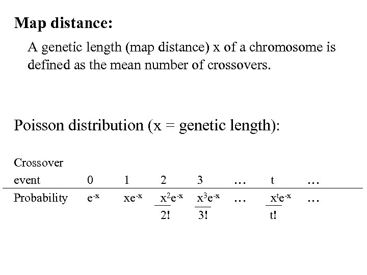Map distance: A genetic length (map distance) x of a chromosome is defined as the mean number of crossovers. Poisson distribution (x = genetic length): Crossover event Probability 0 e-x 1 xe-x 2 x 2 e-x 2! 3 x 3 e-x 3! … … t xte-x t! … …

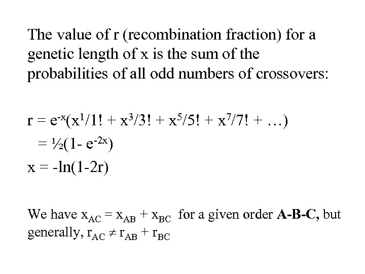The value of r (recombination fraction) for a genetic length of x is the sum of the probabilities of all odd numbers of crossovers: r = e-x(x 1/1! + x 3/3! + x 5/5! + x 7/7! + …) = ½(1 - e-2 x) x = -ln(1 -2 r) We have x. AC = x. AB + x. BC for a given order A-B-C, but generally, r. AC r. AB + r. BC

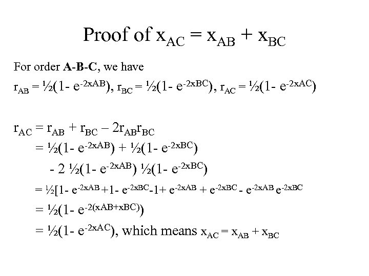Proof of x. AC = x. AB + x. BC For order A-B-C, we have r. AB = ½(1 - e-2 x. AB), r. BC = ½(1 - e-2 x. BC), r. AC = ½(1 - e-2 x. AC) r. AC = r. AB + r. BC – 2 r. ABr. BC = ½(1 - e-2 x. AB) + ½(1 - e-2 x. BC) - 2 ½(1 - e-2 x. AB) ½(1 - e-2 x. BC) = ½[1 - e-2 x. AB +1 - e-2 x. BC-1+ e-2 x. AB + e-2 x. BC - e-2 x. AB e-2 x. BC = ½(1 - e-2(x. AB+x. BC)) = ½(1 - e-2 x. AC), which means x. AC = x. AB + x. BC

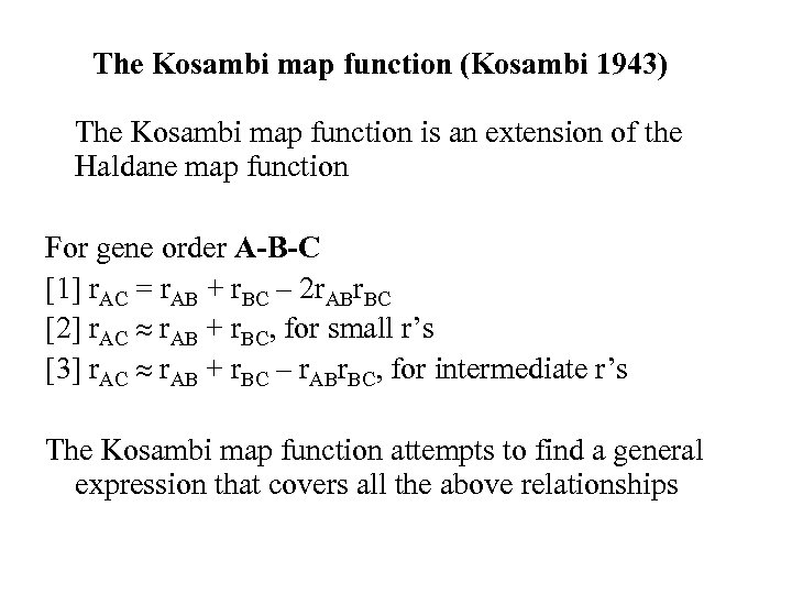The Kosambi map function (Kosambi 1943) The Kosambi map function is an extension of the Haldane map function For gene order A-B-C [1] r. AC = r. AB + r. BC – 2 r. ABr. BC [2] r. AC r. AB + r. BC, for small r’s [3] r. AC r. AB + r. BC – r. ABr. BC, for intermediate r’s The Kosambi map function attempts to find a general expression that covers all the above relationships

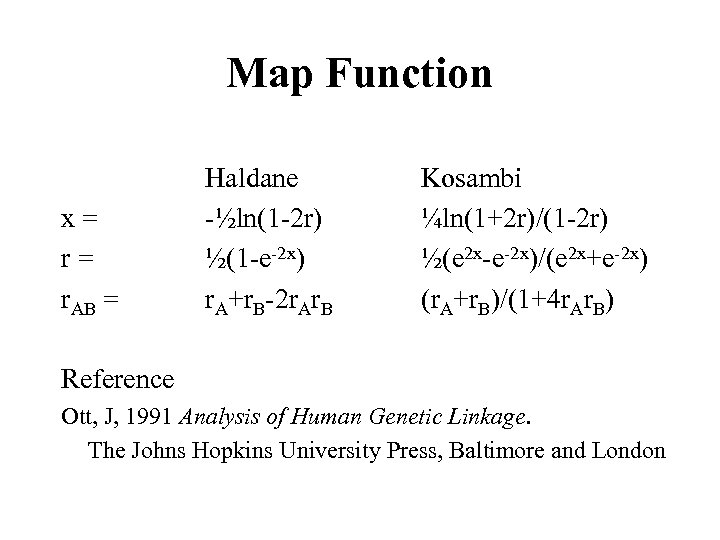Map Function x= r= r. AB = Haldane -½ln(1 -2 r) ½(1 -e-2 x) r. A+r. B-2 r. Ar. B Kosambi ¼ln(1+2 r)/(1 -2 r) ½(e 2 x-e-2 x)/(e 2 x+e-2 x) (r. A+r. B)/(1+4 r. Ar. B) Reference Ott, J, 1991 Analysis of Human Genetic Linkage. The Johns Hopkins University Press, Baltimore and London

Construction of genetic maps • The Lander-Green algorithm -- a hidden Markov chain • Genetic algorithm

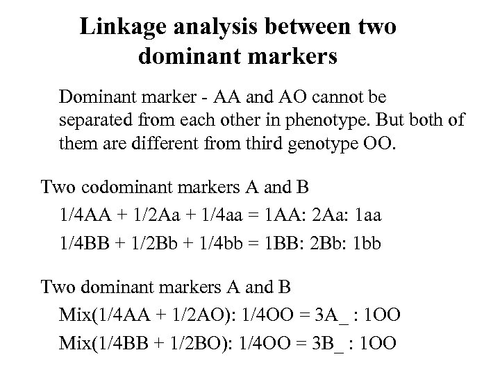Linkage analysis between two dominant markers Dominant marker - AA and AO cannot be separated from each other in phenotype. But both of them are different from third genotype OO. Two codominant markers A and B 1/4 AA + 1/2 Aa + 1/4 aa = 1 AA: 2 Aa: 1 aa 1/4 BB + 1/2 Bb + 1/4 bb = 1 BB: 2 Bb: 1 bb Two dominant markers A and B Mix(1/4 AA + 1/2 AO): 1/4 OO = 3 A_ : 1 OO Mix(1/4 BB + 1/2 BO): 1/4 OO = 3 B_ : 1 OO

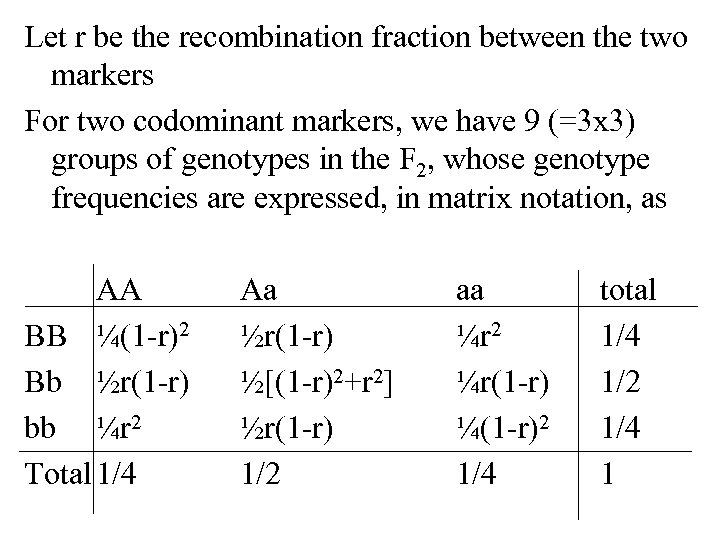Let r be the recombination fraction between the two markers For two codominant markers, we have 9 (=3 x 3) groups of genotypes in the F 2, whose genotype frequencies are expressed, in matrix notation, as AA BB ¼(1 -r)2 Bb ½r(1 -r) bb ¼r 2 Total 1/4 Aa ½r(1 -r) ½[(1 -r)2+r 2] ½r(1 -r) 1/2 aa ¼r 2 ¼r(1 -r) ¼(1 -r)2 1/4 total 1/4 1/2 1/4 1

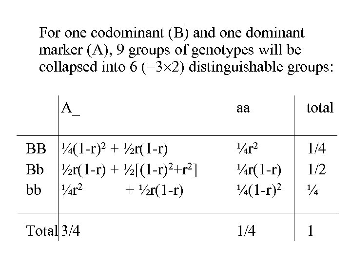For one codominant (B) and one dominant marker (A), 9 groups of genotypes will be collapsed into 6 (=3 2) distinguishable groups: A_ aa total BB ¼(1 -r)2 + ½r(1 -r) Bb ½r(1 -r) + ½[(1 -r)2+r 2] bb ¼r 2 + ½r(1 -r) ¼r 2 ¼r(1 -r) ¼(1 -r)2 1/4 1/2 ¼ Total 3/4 1

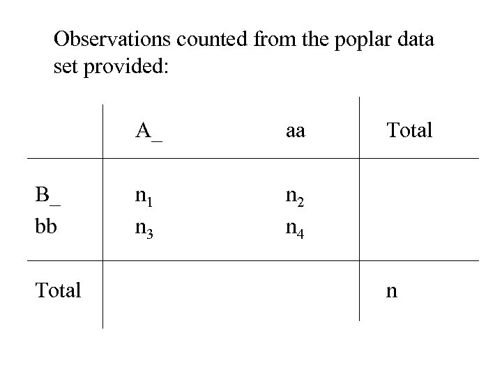
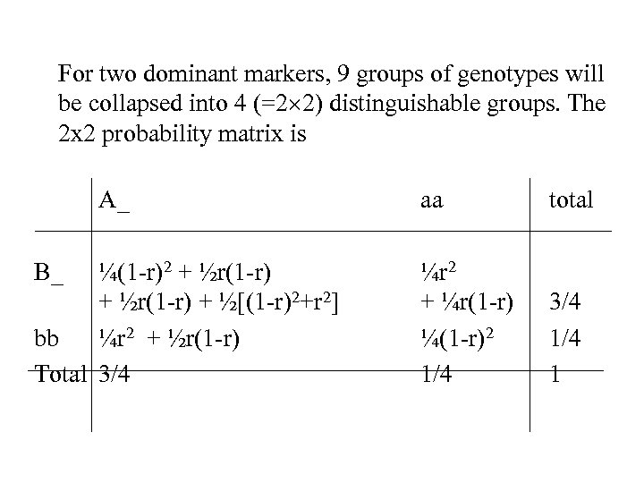For two dominant markers, 9 groups of genotypes will be collapsed into 4 (=2 2) distinguishable groups. The 2 x 2 probability matrix is A_ B_ ¼(1 -r)2 + ½r(1 -r) + ½[(1 -r)2+r 2] bb ¼r 2 + ½r(1 -r) Total 3/4 aa total ¼r 2 + ¼r(1 -r) ¼(1 -r)2 1/4 3/4 1

Observations counted from the poplar data set provided: A_ B_ bb Total aa n 1 n 3 Total n 2 n 4 n

Expected numbers of recombinant gametes (the number of r) B_ bb A_ c 1 c 2 aa c 2 0 where c 1 = [2 ½r 2+1 r(1 -r)]/[½r 2+r(1 -r)+¾(1 -r)2] c 2 = [2 ¼r 2+1 ½r(1 -r)]/[¼r 2+½r(1 -r)] (1) (2) Based on the definition of r (the proportion of recombinant gametes over all gametes), we have r^ = (c 1 n 1 + c 2 n 2 + c 3 n 3) /2 n (3) Equations (1) and (2) are for the E step, whereas Equation (3) is for the M step.