5da62eb24b7b44eefec5d46f138b3b2f.ppt
- Количество слайдов: 46


 modeling 04/04/2016")
Generative (Bayesian) modeling 04/04/2016
: David M. Blei Andrew Y. Ng, Michael I. Jordan, Ido")
Slides by (credit to): David M. Blei Andrew Y. Ng, Michael I. Jordan, Ido Abramovich, L. Fei-Fei, P. Perona, J. Sivic, B. Russell, A. Efros, A. Zisserman, B. Freeman, Tomasz Malisiewicz, Thomas Huffman, Tom Landauer and Peter Foltz, Melanie Martin, Hsuan-Sheng Chiu, Haiyan Qiao, Jonathan Huang Thank you!

Generative modeling • unsupervised learning • … beyond clustering • How can we describe/model the world for the computer? • Bayesian networks!
 whose nodes represent random variables • Arcs")
Bayesian networks • Directed acyclic graphs (DAG) whose nodes represent random variables • Arcs represent (directed) dependence between random variables
 variables")
Bayesian networks • Filled nodes: observable variables • Empty nodes: hidden (not observable) variables Zi wi 1 w 2 i w 3 i w 4 i

Collapsed notation of Bayesian networks • Frames indicates multiplications – E. g. N features and M instances: Zi wi 1 w 2 i w 3 i w 4 i
 modeling Find the parameters of the given model which explains/reconstruct the observed")
Generative (Bayesian) modeling Find the parameters of the given model which explains/reconstruct the observed data DATA Model „Generative story”

Model „Generative story” • Model = Bayesian network • The structure of the network is given by the human engineer • The form of the nodes’ distribution (conditioned on their parents) is given as well • The parameters of the distributions have to be estimated from data

Parameter estimation in Bayesian network – only observable variables • Bayesian network assumes that the variables only (directly) dependent from their parents → parameter estimation at each node can be carried out separetly • Maximum Likelihood (or Bayesian estimation)
 • The extension of Maximum Likelihood parameter estimation if hidden variables are")
Expectation-Maximisation (EM) • The extension of Maximum Likelihood parameter estimation if hidden variables are present • We search for the parameter vector Φ which maximises the likelihood of the joint of observable variables X and hidden ones Z
 • Iterative algorithm. Step l: – (E)xpectation step: estimate the values of")
Expectation-Maximisation (EM) • Iterative algorithm. Step l: – (E)xpectation step: estimate the values of Z (calculate expected values) using Φl – (M)aximization step: Maximum likelihood estimetion by using Z

EM example There are two coins. We drop them together but we can observe only the sum of the heads: h(0)=4 h(1)=9 h(2)=2 What is the bias of the coins? Φ 1=P 1(H), Φ 2=P 2(H) ?

EM example a single z hidden variable: what is the proportion of the first coin out of h(1)=9 init Φ 10=0. 2 Φ 20=0. 5 E-step

EM example M-step

Text classification/clustering • E. g. recognition of documents’ topic or clustering images based on their content • „Bag-of-words model” • The term-document matrix:

Image Bag-of-”words”

• N documents: D={d 1, … , d. N} • The dictionary consists of M words – W={w 1 , … , w M} • The size of the term-document matrix is N * M and it contains the number of occurances of a certain word in a certain document

Drawbacks of the bag-of-words model – Word order is ignored – Synonyms: We refer to a concept (object) by multiple words, e. g: tired-sleepy → low recall – Polysemy: most of words have multiple senses, pl: bank, chips → low precision

Document clustering – unigram model • Let’s assign a „topic” to each document • The topics are hidden variables

Generative story of „unigram model” How documents generate? 1. „Drop” a topic (and a size) TOPIC 2. For each word position drop a word according to the topic’s distribution Word . . . Word

Unigram model Zi wi 1 w 2 i w 3 i w 4 i Each M documents, p Drop a topic z. p Drop a word (independently from the others) from a multinomial distribution conditiond on z

EM for clustering • E-step • M-step

p. LSA Probabilistic Latent Semantic Analysis • We assign a distribution of topics to each of the document • Topics still have a distrbution over words • The distributions found are interpretable

Relation to clustering… • A document can belong to multiple clusters • We’re interested in the distribution of topics rather than pushing each doc into a cluster → more flexible

Generative story of p. LSA How documents generate? 1. 2. 3. Generate the document’s topic distribution For each word position drop a topic from the doc’s topic distribution drop a word according to the topic’s distribution TOPIC . . . TOPIC word . . . word
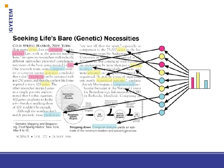

Example mo loan y m bank DOCUMENT 1: money 1 bank 1 loan 1 river 2 stream 2 bank 1 money 1 river 2 bank 1 money 1 bank 1 loan 1 money 1 stream 2 bank 1 money 1 bank 1 loan 1 river 2 stream 2 bank 1 money 1 river 2 bank 1 money 1 bank 1 loan 1 bank 1 money 1 stream 2 . 8 ba nk loan bank ey on ne . 2 TOPIC 1 riv er . 3 stream str eam ban k r river nk ba TOPIC 2 . 7 DOCUMENT 2: river 2 stream 2 bank 2 money 1 loan 1 river 2 stream 2 loan 1 bank 2 river 2 bank 1 stream 2 river 2 loan 1 bank 2 stream 2 bank 2 money 1 loan 1 river 2 stream 2 bank 2 money 1 river 2 stream 2 loan 1 bank 2 river 2 bank 2 money 1 bank 1 stream 2 river 2 bank 2 stream 2 bank 2 money 1
 ? TOPIC 1 ? TOPIC 2 DOCUMENT 1: money?")
Parameter estimation (model fitting, training) ? TOPIC 1 ? TOPIC 2 DOCUMENT 1: money? bank? loan? river? stream? bank? money? river? bank? money? bank? loan? money? stream? bank? money? bank? loan? river? stream? bank? money? river? bank? money? bank? loan? bank? money? stream? ? DOCUMENT 2: river? stream? bank? money? loan? river? stream? loan? bank? river? bank? stream? river? loan? bank? stream? bank? money? loan? river? stream? bank? money? river? stream? loan? bank? river? bank? money? bank? stream? river? bank? stream? bank? money?

p. LSA Observable data Term distributions over topics Topic distributions For documents Slide credit: Josef Sivic
")
Latent semantic analysis (LSA)

Generative story of p. LSA How documents generate? 1. 2. 3. Generate the document’s topic distribution For each word position drop a topic from the doc’s topic distribution drop a word according to the topic’s distribution TOPIC . . . TOPIC word . . . word

p. LSA modell d zd 1 zd 2 zd 3 zd 4 wd 1 wd 2 wd 3 wd 4 For each document d and word position: – For each word position drop a topic from the doc’s topic distribution – drop a word according to the topic’s distribution
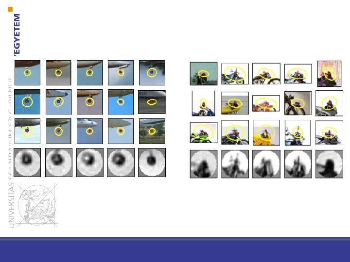
 d D z w N “eye” Sivic et al.")
p. LSA for images (example) d D z w N “eye” Sivic et al. ICCV 2005

p. LSA – parameter estimation
")
p. LSA – E-step What is the expected value of hidden variables (topics z) if the parameter values are fixed
")
p. LSA – M-step We use the values of hidden variables p(z|d, w)

EM algorithm • It can converge to local optimum • Stopping condition?

Approximate inference • The E-step in huge networks is unfeasible • There approaches which are fast but do only approximate inference (=E-step) rather than exact one • The most popular approximate inferece method is: 1. Drop samples according to Bayesian network 2. The average of the samples can be used as expected values of hidden variables
 • MCMC is an approximate inference method •")
Markov Chain Monte Carlo method (MCMC) • MCMC is an approximate inference method • The samples are not independent from each other but they are generated one by one based on the previous sample (form a chain) • Gibbs sampling is the most famous MCMC method: – The next sample is generated by fixing all but variables and drop a value for the non-fixed one conditioned on the other ones

Outlook

Drawbacks of p. LSA • It can be recalculated from scratch if a new document arrives • The number of parameters increases as the function of the number of instances • d is just an index, it doesn’t fit well into the generative story

1990 1999 2003

2010

An even more complex task Recognise objects inside images without any supervision After training the model can be applied for unknown images as well
 modeling enables to define any description/model of the world with")
Summary • Generative (Bayesian) modeling enables to define any description/model of the world with any complexity (clustering is only an example for it) • EM algorithm is a general tool for solving parameter estimation problems where latent variables is incorporated
5da62eb24b7b44eefec5d46f138b3b2f.ppt