40593ed57d0acbe5f2166afb9c88becf.ppt
- Количество слайдов: 71


Generation Adequacy Planning LOLE/LOLP Study Seminar by Gene Preston g. preston@ieee. org December 6, 2002

Seminar Purpose • Show the methodology for calculating the reliability indices using graphics and examples • Define terms used in reliability studies such as LOLE, LOLP, EUE, FOR, PFOR, pdf, etc. • Provide information to stakeholders concerning input data and interpretation of study results for single area and multi-area studies

Generation Adequacy Study Objectives • Ensure installed generation reserve is sufficient • Test the sensitivity of study parameters
 ~ Pmax time at")
pdf = probabilistic density function of a typical generator f(x) ~ Pmax time at each MW level f(x) total area = 1 0 x - megawatts (MW) forced out of service See notes for each slide for more information. Pmax
 F(x) 1. 5 x 1")
Cumulative distribution function of the pdf random variables f(x) F(x) 1. 5 x 1 - area = value expected value or mean value F(x) = 1 - Pr[generation MW ≤ x] = Pr[generation MW > x]

Combination of two generator pdfs using convolution

Representation of pdfs with discrete states x 1 gen 1 Pr x 2 gen 2 Pr . 125 . 1653 . 375 . 25 . 375 . 2123 . 625 . 2725 . 875 . 3499

Take all combinations of Pr’s and MW’s X Pr 0. 25 0. 0413250 0. 0944000 0. 75 0. 1625250 1. 00 0. 2500000 1. 25 0. 2086750 1. 50 0. 1556000 1. 75 0. 0874750
. 8")
Representation of pdfs with discrete states (one generator with states: 0, Derated, Pmax). 8 f(x) . 1 PFOR . 1 FOR 0 x - MW Derated Pmax

Generator failure as an exponential function of time 1 probability of failure = t = 0 1/λ mean time to failure probability of failure = 1 – exp(–λt)
 derived from λ and µ up µ Pr[unit")
Steady state FOR (forced outage rate) derived from λ and µ up µ Pr[unit is up] = P 1 λ down Pr[unit is down] = P 0 λ = failure rate µ = repair rate µP 0 = λP 1 and P 0 + P 1 = 1 gives P 0 = λ / (λ + µ) also FOR = P 0 = Pr[down] FOR = per unit down time

Markov representation of a 3 -state generator Pmax P 1 µ 1 λ 2 λ 1+λ 2 –µ 2 –µ 1 P 1 0 µ 2 MW –λ 2 µ 2+λ 3 –µ 3 P 2 0 P 2 Pder MW λ 3 µ 3 0 MW P 3 1 1 P 3 1 PFOR = per unit derated time (partial forced outage rate) FOR = per unit down time

Use of the Markov process to represent three two-state generators U 9 U 1 4 U 1 2. 33 1 D D D unit 1 FOR=. 1 10 MW unit 2 FOR=. 2 15 MW unit 3 FOR=. 3 20 MW

Markov representation of three generators P 1 2. 33 UUU 9 4 1 P 2 P 3 UUD 4 1 1 2. 33 UDU 2. 33 9 9 1 P 5 1 4 1 1 P 4 P 6 UDD DUD 9 1 2. 33 1 P 8 DDD P 7 DDU 4 1 DUU 1

Markov representation of three generators 3 -2. 3 -4 0 -9 0 0 0 -1 4. 3 0 -4 0 -9 0 0 -1 0 6 -2. 3 0 0 -9 0 0 -1 -1 7. 3 0 0 0 -9 -1 0 0 0 11 -2. 3 -4 0 0 -1 0 0 -1 12. 3 0 -4 0 0 -1 0 14 -2. 3 1 1 P 1 P 2 P 3 P 4 P 5 P 6 P 7 P 8 0 0 0 0 1

Markov representation of three generators P 1 P 2 P 3 P 4 P 5 P 6 P 7 P 8 . 504 45 MW. 216 25 MW. 126 30 MW. 054 10 MW. 056 35 MW. 024 15 MW. 014 20 MW. 006 0 MW

Use of a binary tree for the three generators to perform the convolution process Individual States Gen 1 Pr ΣPr 20. 7 -- 45. 504 15. 8 0. 3 -- 25. 216 35. 056 . 560 0. 2 20. 7 -- 30. 126 . 686 25. 216 . 902 20. 7 -- 35. 056 10. 9 Gen 2 Gen 3 MW Cumulative Pr 20. 014 . 916 15. 8 0. 3 -- 15. 024 . 940 0. 2 20. 7 -- 20. 014 10. 054 . 994 0. 3 -- 10. 054 0. 1 0. 3 -- 0. 006 MW sort 0. 006 1. 000

Graph of the 3 generator cumulative distribution for the probability that generation MW is > x). 994 1. 0. 9. 8. 7. 6 Pr. 5. 4. 3. 2. 1 0 . 940 . 916. 902 load not served. 686. 560 . 504 generation . 000 0 5 10 15 20 25 30 x (MW) 35 40 45 50

Unsuitability of the binary tree and Markov methods for large systems A system with 400 two-state generators has a total of: 400 2 120 10 states (combinations) This is greater than the number of atoms in the universe (~1080)!

The same cumulative distribution can be created one generator at a time. The function is updated as each generator is added. . 994 1. 0. 9. 8. 7. 6 Pr. 5. 4. 3. 2. 1 0 . 940 . 916. 902 load not served. 686. 560 . 504 generation . 000 0 5 10 15 20 25 30 x (MW) 35 40 45 50

Starting with a blank distribution 1. 0. 9. 8. 7. 6 Pr. 5. 4. 3. 2. 1 0 load not served 0 5 10 15 20 25 30 x (MW) 35 40 45 50

Cumulative distribution for generator 1 = {10 MW, FOR=. 1} ∞ 1. 0. 9. 8. 7. 6 Pr. 5. 4. 3. 2. 1 0 . 900 load not served . 000 0 5 10 15 20 25 30 x (MW) 35 40 45 50
 and")
Adding generator 2 scales and shifts the initial distribution for Pr=. 8 (up) and Pr=. 2 (down) generator 2 = {15 MW, FOR=. 2} 1. 0. 9. 8. 7. 6 Pr. 5. 4. 3. 2. 1 0 1. 00 x. 8 =. 80. 900 x. 8 =. 72 . 900 x. 2 =. 18 0 5 10 15 20 25 30 x (MW) 35 40 45 50

Summing the two curves gives the combined generators 1 and 2 cumulative distribution 1. 0. 9. 8. 7. 6 Pr. 5. 4. 3. 2. 1 0 . 80+. 18=. 98. 80. 72 load not served generation . 000 0 5 10 15 20 25 30 x (MW) 35 40 45 50
 and Pr=.")
Adding generator 3 scales and shifts the distribution for Pr=. 7 (up) and Pr=. 3 (down) generator 3 = {20 MW, FOR=. 3} 1. 0. 9. 8. 7. 6 Pr. 5. 4. 3. 2. 1 0 1. 00 x. 7=. 700 . 98 x. 7=. 686. 80 x. 7=. 56. 72 x. 7=. 504 . 98 x. 3=. 294. 80 x. 3=. 24. 72 x. 3=. 216 0 5 10 15 20 25 30 x (MW) 35 40 45 50

Summing the two curves gives the combined generators 1, 2, and 3 cumulative distribution (same curve as the one using a binary tree). 294+. 700=. 994 2 load not served 90 6=. . 6 8 6+. 2 1 . 6+ . + 24 . 9 1. 7 = = 70 6 0 94. . 2 1 1. 0. 9. 8. 7. 6 Pr. 5. 4. 3. 2. 1 0 . 686. 560 . 504 generation . 000 0 5 10 15 20 25 30 x (MW) 35 40 45 50

Binary tree graph of the 3 generator cumulative distribution for the probability that generation is available at x MW. 994 1. 0. 9. 8. 7. 6 Pr. 5. 4. 3. 2. 1 0 . 940 . 916. 902 load not served. 686. 560 . 504 generation . 000 0 5 10 15 20 25 30 x (MW) 35 40 45 50
![Cumulative distribution Pr[generation is up] represented in discrete 1 MW steps 1. 0. 9.](https://present5.com/presentation/40593ed57d0acbe5f2166afb9c88becf/image-28.jpg "Cumulative distribution Pr[generation is up] represented in discrete 1 MW steps 1. 0. 9.")
Cumulative distribution Pr[generation is up] represented in discrete 1 MW steps 1. 0. 9. 8. 7. 6 Pr. 5. 4. 3. 2. 1 0 load not served generation 0 5 10 15 20 25 30 x (MW) 35 40 45 50
![Flip the function over and backwards and the distribution represents Pr[generation out of svc]](https://present5.com/presentation/40593ed57d0acbe5f2166afb9c88becf/image-29.jpg "Flip the function over and backwards and the distribution represents Pr[generation out of svc]")
Flip the function over and backwards and the distribution represents Pr[generation out of svc] This is the COPT or Capacity Outage Probability Table 1. 0. 9. 8. 7. 6 Pr. 5. 4. 3. 2. 1 0 . 496 . 440. 314 load not served 45 40 35 30 . 098. 084. 060 25 20 15 x (MW) 10 . 006 . 000 5 0
![Representation of Pr[gen out of service] as piecewise linear increments 1. 0. 9. 8.](https://present5.com/presentation/40593ed57d0acbe5f2166afb9c88becf/image-30.jpg "Representation of Pr[gen out of service] as piecewise linear increments 1. 0. 9. 8.")
Representation of Pr[gen out of service] as piecewise linear increments 1. 0. 9. 8. 7. 6 Pr. 5. 4. 3. 2 load not served. 1 0 0 5 10 15 20 25 30 x (MW) 35 40 45 50
![Representation of Pr[gen out of service] as piecewise quadratic increments 1. 0. 9. 8.](https://present5.com/presentation/40593ed57d0acbe5f2166afb9c88becf/image-31.jpg "Representation of Pr[gen out of service] as piecewise quadratic increments 1. 0. 9. 8.")
Representation of Pr[gen out of service] as piecewise quadratic increments 1. 0. 9. 8. 7. 6 Pr. 5. 4. 3. 2 load not served. 1 0 0 5 10 15 20 for any 3 points, interpolate between the left two points 25 30 x (MW) 35 40 45 50
 and piecewise")
Relative per unit error introduced by numerous interpolations of piecewise linear (PL) and piecewise quadratic (PQ) distributions PL x=30% PQ x=20%

LOLE – loss of load expectation EUE – expected unserved energy EUE = MWH not served (for each hour in the study) 1. 0. 9. 8. 7. 6 Pr. 5. 4. 3. 2. 1 0 . 994. 940 . 916 . 902 LOLE for one day = 1 - Pr[gen up] = Pr[load loss] = 1 -. 56 =. 44 d/y . 686. 560 . 504 generation 0 5 10 15 20 25 30 35 40 45 50 MW x – MW (daily or hourly)

LOLP – loss of load probability 1. 0. 9. 8. 7. 6 Pr. 5. 4. 3. 2. 1 0 LOLP (for a week) = 1 - Pr[gen up] = Pr[load loss] = 1 -. 56 =. 44 . 994. 940 . 916 . 902 . 686. 560 . 504 generation annual LOLP = 1 - i(Pr[gen up]i) for all i weeks 0 5 10 15 20 25 30 35 40 45 x – MW weekly peak demand 50 MW
. 994 1.")
Representing load uncertainty (each hour is a Normal distribution of MW values). 994 1. 0. 9. 8. 7. 6 Pr. 5. 4. 3. 2. 1 0 . 940 . 916 . 902 . 686. 560 . 504 generation 0 5 10 15 20 25 30 35 40 45 x – MW (daily or hourly) 50 MW

Generation scheduled maintenance generator # insufficient reserve? 1 xxx 2 xxx 3 4 xxxxx 5 summer 6 xxx 7 8 xxxx 9 xxx 10 xxxx 11 1 5 10 15 20 25 30 35 40 45 50 52 week # during the year

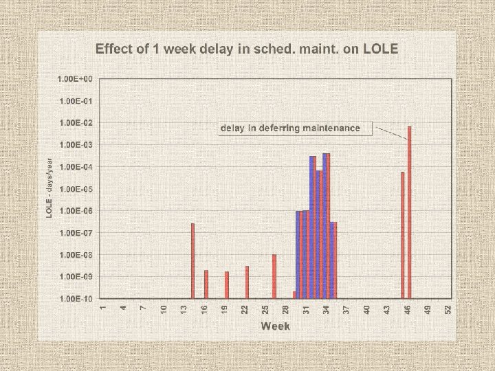
Generation scheduled maintenance reduces available generation – increases LOLE generator installed MW before maintenance MW demand 1 5 planning reserve with maint insufficient reserve 10 15 20 25 30 35 40 week # during the year 45 50 52

Generation scheduled maintenance to minimize overall LOLE generator installed MW before maintenance with maint MW demand 1 5 planning reserve 10 15 20 25 30 35 40 week # during the year 45 50 52

Automatic scheduled maintenance methodology to minimize LOLE 1. Sort the MW unit sizes from largest to smallest. 2. Place the largest MW generator in a time slot with the greatest unused reserve margin. 3. Place the next largest generator in a time slot with the greatest unused reserve margin. 4. Repeat step 3 until all units are scheduled.

1999 load shape

1999 load shape
 forced out of service and derated actual more generators ~5000 MW")
ERCOT generation (MW) forced out of service and derated actual more generators ~5000 MW ~6% ~9000 MW ~11% 12. 5% 0 2000 4000 6000 8000 10000 12000

DC tie considerations • probability of a DC tie failure is nearly 0 • probability of generation supply being available in the other region is expected to be nearly 1 • transmission constraints in the other region may reduce the probability of DC tie capability to less than 1 • DC tie capacity can be included or excluded from the LOLP calculations (affects the LOLE) • DC tie capacity may or may not be used to serve firm load in ERCOT (affects the reserve)

DC tie considerations DC tie in LOLP calculations Yes No LOLP: 100% DC MW CDR : X MW gen 12. 5% reserve LOLP: 100% DC MW DC tie with 0 MW firm generation CDR : X MW gen 11% x=0 to 12. 5% for x=all firm DC tie with X MW firm generation LOLP: X MW DC LOLP: 0 MW DC CDR : 0 MW gen 11% reserve 12. 5% reserve

Switchable generation considerations • Switchable generation capability must be available to ERCOT when called upon. • The same switchable MWs must be used in both the reserve calculation and the LOLP calculation.

Self-serve generation considerations • Currently, both the self serve generation and self serve load (840 MW in the previous study) are omitted from the CDR and the LOLP calculations. • Alternately, the self serve generation and load could be included with the CDR and LOLP calculations with a negligible effect on LOLE. • Currently, self serve generation and load are included in the transmission load flow analysis as fixed MW values with 100% availability.

Interruptible load considerations • The load can be modeled as two components, firm plus interruptible (i. e. two forecasts) • The LOLE for serving firm load can be calculated by using only the forecast for firm load in the computer simulation. • The LOLE for interruptible load can be calculated by using a forecast of firm load plus interruptible load in the computer simulation and then subtracting the LOLE results obtained for the firm load forecast.
")
Data needed to perform single-area LOLP studies • hourly ERCOT loads for the (annual) study period (historical year hourly loads are scaled) • the annual peak demand forecast and the percentage of interruptible load • percentage of load forecast uncertainty • each generator’s seasonal MW (Pmax) capability, fuel type, type of unit, and maintenance periods (by beginning and ending week numbers or by total weeks needed) • FOR and DFOR of generator types such as gas, coal, nuclear, hydro, wind, etc. • identification of self-serve MW by generator

Single Area Output Reports – Input Data SINGLE AREA GENERATOR DATA: SEASONAL CAPACITIES UNIT AREA WINT SPNG SUMM FALL NAME MW MW ----------- ---STP 1 ERCOT 1311 STP 2 ERCOT 1311 CMPK 1 G ERCOT 1161 CMPK 2 G ERCOT 1161 DOW 1 ERCOT 986 986 DOW 2 ERCOT 917 917 DEC 1 G ERCOT 818 818 THSE 2 G ERCOT 818 818 LIM 1 ERCOT 744 744 LIM 2 ERCOT 744 744 MTNLK 1 G ERCOT 727 727 MTNLK 2 G ERCOT 727 727 MTNLK 3 G ERCOT 727 727 MOSES 3 G ERCOT 726 726 CB 3 ERCOT 703 703 DC-EAST ERCOT 700 700 Weeks 1 -9 49 -52 Weeks 10 -21 Weeks 22 -37 CDR CAP % --100 100 100 100 0 Weeks 38 -48 FORCED PARTIAL-OUTAGE RATE DERATNG RATE % % % ------6. 90 2. 30 5. 50 10. 00 6. 70 0. 00 4. 22 2. 90 19. 00 6. 70 0. 00 0. 01 0. 00 SCHEDULED UNAVAILABLE B 1 D 1 B 2 D 2 -- -- -- -5 4 0 0 4 4 0 0 11 4 0 0 3 12 0 0 7 4 0 0 3 12 0 0 48 4 0 0 13 4 0 0 3 12 0 0 43 4 0 0 48 4 0 0 49 4 1 8 43 4 0 0 13 4 0 0 3 12 0 0

Single Area Output Reports – Maintenance AUTOMATIC MAINTENANCE OF 12 LONG & 4 SHORT WEEKS SCHEDULED UNAVAILABLE: -WINTER- ---SPRING--- ----SUMMER----FALL--- WIN UNIT AREA JAN FEB MAR APR MAY JUN JUL AUG SEP OCT NOV DEC NAME week: 11111222223333344444555 -------12345678901234567890123456789012 PB 5 G ERCOT ooooooo. . . . ooooo PB 6 G ERCOT. . . . oooo. MRGN 2 G ERCOT oo. . . . ooooo MRGN 4 G ERCOT. . . . oooo. . MRGN 5 G ERCOT. . . . oooo. MRGN 3 G ERCOT oo. . . . ooooo

Single Area Output Reports – CDR WEEK ---16 17 18 19 20 21 22 23 24 25 26 27 28 29 30 31 32 33 34 35 36 37 38 39 40 CAPACITY MW -------80223. 80223. 80223. OUT-OF-SVC MW -------0. 0. 0. 0. AVAILABLE MW -------80223. 80223. 80223. PEAK LOAD MW -------0. 35344. 49251. 52755. 53323. 54975. 60222. 57907. 55546. 57007. 63446. 62549. 62641. 64447. 67662. 67691. 70378. 69615. 70535. 67195. 63388. 58919. 61987. 59018. 0. RESERVE MW -------80223. 44879. 30972. 27468. 26900. 25248. 20001. 22316. 24676. 23216. 16777. 17673. 17582. 15776. 12561. 12532. 9845. 10607. 9688. 13027. 16835. 21303. 18236. 21205. 80223. RESERVE % ------0. 0 127. 0 62. 9 52. 1 50. 4 45. 9 33. 2 38. 5 44. 4 40. 7 26. 4 28. 3 28. 1 24. 5 18. 6 18. 5 14. 0 15. 2 13. 7 19. 4 26. 6 36. 2 29. 4 35. 9 0. 0 WEEK BEGINS -----APR 18 APR 25 MAY 2 MAY 9 MAY 16 MAY 23 MAY 30 JUN 6 JUN 13 JUN 20 JUN 27 JUL 4 JUL 11 JUL 18 JUL 25 AUG 1 AUG 8 AUG 15 AUG 22 AUG 29 SEP 5 SEP 12 SEP 19 SEP 26 OCT 3

Single Area Output Reports – LOLE Results WEEK PEAK LOAD MW -----16 0. 17 35344. 18 49251. 19 52755. 20 53323. 21 54975. 22 60222. 23 57907. 24 55546. 25 57007. 26 63446. 27 62549. 28 62641. 29 64447. 30 67662. 31 67691. 32 70378. 33 69615. 34 70535. 35 67195. 36 63388. 37 58919. 38 61987. 39 59018. 40 0. ANNUAL 70535. RESERVE % ------0. 0 127. 0 62. 9 52. 1 50. 4 45. 9 33. 2 38. 5 44. 4 40. 7 26. 4 28. 3 28. 1 24. 5 18. 6 18. 5 14. 0 15. 2 13. 7 19. 4 26. 6 36. 2 29. 4 35. 9 0. 0 13. 7* LOSS OF LOAD EXPECTATION = WEEKLY PROBABILITY LOAD>GENR -. --3 --6 --9 -12 -150. 0000000000000000 0. 0000000692 0. 0000000000000000 0. 000013815166 0. 000001051571 0. 000001375059 0. 0000000208146472 0. 0000393594360814 0. 0000418127666276 0. 0053711529435669 0. 0015578843676685 0. 0068264952639734 0. 0000147424748045 0. 000011738335 0. 000000008 0. 00000194574 0. 000000011 0. 00000000 0. 0137945421779943 HOURLY UNSERVED WEEK MWH BEGINS ----. --3 --6 --9 -----0. 00000 APR 18 0. 00000 APR 25 0. 00000 MAY 2 0. 00000 MAY 9 0. 00000 MAY 16 0. 00000 MAY 23 0. 00000 MAY 30 0. 00000 JUN 6 0. 00000 JUN 13 0. 00000 JUN 20 0. 0000009830 JUN 27 0. 0000000560 JUL 4 0. 0000000719 JUL 11 0. 0000123400 JUL 18 0. 0782425020 JUL 25 0. 0886081361 AUG 1 11. 2483312958 AUG 8 2. 7090544949 AUG 15 7. 4071353617 AUG 22 0. 0100945754 AUG 29 0. 0000010857 SEP 5 0. 00000 SEP 12 0. 000072 SEP 19 0. 00000 SEP 26 0. 00000 OCT 3 21. 5414809098 (* INSTALLED) 0. 019290 DAYS/YR USING DAILY PEAK LOADS AND NO LOAD UNCERTAINTY 0. 001565 DAYS/YR USING HOURLY LOADS AND NO LOAD UNCERTAINTY
 – requires the development of an")
Transmission model considerations • Simplified transmission network (NARP) – requires the development of an equivalent – computationally fast – questionable circuit flow results • Full transmission network (PLF) – eliminates the need to develop an equivalent – computationally fast if PDFs are used – results are in agreement with AC load flow

Transmission PDFs from AC load flows PDF = power distribution factor = MW ckt flow / MW power transfer difference in two shift factors flow load buses gen
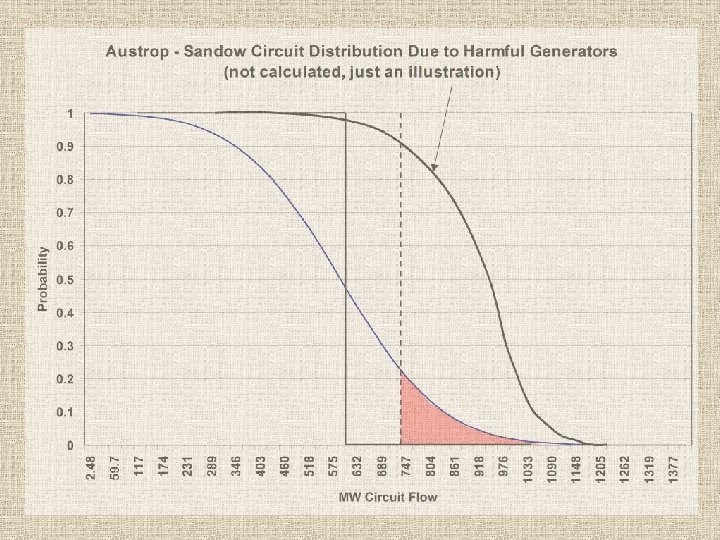

Harmful Generators for Austrop-Sandow Ckts PDFs for ckt: 3429 SANDOW 345 221 LOSTPN 2 -0. 1734601 load 222 LOSTPN 3 -0. 1734599 load 220 LOSTPN 1 -0. 1734593 load 257 BEP GT 2 -0. 1689710 load 256 BEP GT 1 -0. 1689707 load 258 BEP ST 1 -0. 1689678 load 223 FPP G 1 -0. 1501281 load 224 FPP G 2 -0. 1501194 load 225 FPP G 3 -0. 1498940 load 229 HAYSN 4 -0. 1423499 load 228 HAYSN 3 -0. 1423486 load 226 HAYSN 1 -0. 1423371 load 227 HAYSN 2 -0. 1423371 load 247 MCQUEE 06 -0. 1342581 load 322 SANDH G 1 -0. 1341542 load 323 SANDH G 2 -0. 1341542 load 325 SANDH G 4 -0. 1341535 load 324 SANDH G 3 -0. 1341533 load 246 CANYHY 06 -0. 1338861 load 313 DECKR G 2 -0. 1316094 load 312 DECKR G 1 -0. 1315037 load 7040 AUSTRO 34 345 flow bus 7008 flow bus 7009 flow bus 7007 flow bus 7808 flow bus 7807 flow bus 7809 flow bus 7010 flow bus 7011 flow bus 7012 flow bus 7017 flow bus 7016 flow bus 7014 flow bus 7015 flow bus 7605 flow bus 9016 flow bus 9017 flow bus 9019 flow bus 9018 flow bus 7487 flow bus 9001 flow bus 9000 1

More Generator PDFs for Austrop-Sandow 252 250 251 248 253 254 255 261 259 260 315 316 317 314 263 262 264 249 276 153 GUALUP 1 GUALUP 2 SCHUMA 13 GUALUP 4 GUALUP 5 GUALUP 6 RIONO G 3 RIONO G 1 RIONO G 2 DECKR G 4 DECKR G 5 DECKR G 6 DECKR G 3 RIONO G 5 RIONO G 4 RIONO G 6 LAKEWD 06 LAR #3 SAND 4 G SOUTH NORTH WEST HOUSTON -0. 1303046 -0. 1303038 -0. 1302463 -0. 1302456 -0. 1293995 -0. 1293991 -0. 1293990 -0. 1291926 -0. 1291925 -0. 1291662 -0. 1291648 -0. 1291633 -0. 1285502 -0. 1281178 0. 1279722 -0. 1045032 0. 0786292 0. 0504448 -0. 0243481 load load load load load load flow flow flow flow flow flow bus bus bus bus bus area 7802 7800 7801 7609 7805 7812 7810 7811 9003 9004 9005 9002 7814 7813 7815 7624 8288 3432 4 2 1 3

Maximum Flows for Austrop-Sandow Ckts MAXIMUM +/- LINE FLOWS FROM SUMS OF INCREMENTAL GENERATOR FLOWS -------FROM-----3429 SANDOW 345 -------TO-------7040 AUSTRO 34 345 average weighted scale factor = RATG 716 789 BASE -356. 0 +MW -MW 2840. 0 -3269. 3 %ADJ -2. 24 % sum of flows from helpers sum of flows from harmers

Maximum Flow Sources for Austrop-Sandow MAXIMUM CIRCUIT FLOWS WITH ALL CIRCUITS IN SERVICE -------FROM-----3429 SANDOW 345 -------TO-------7040 AUSTRO 34 345 ID RATG PCT 1 716 -446 2 789 -405 1 716 397 2 789 360 -GENERATION-to-LOADLOSTPN 2 18 ->NORTH SAND 4 G 22 ->SOUTH DIST. 252. 232
 static base")
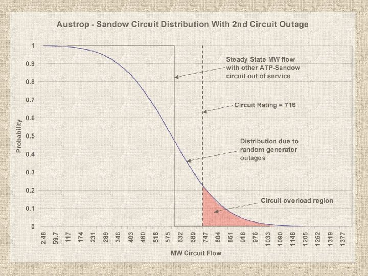
Probabilistic flows on a circuit (in preparation to remove the overloaded portion) static base case flow 1 ckt rating Pr [ flow>x ] overload 0 0 MW

Removing a transmission overload Pr Pr circuit rating p MW shift a binary tree of generation states p ckt overload states p MW shift Pr[loss of gen>x] generation states Pr[ckt MW>x] one circuit’s flows p = Pr[of an individual generation state]

Correlating the removal of a transmission overload with the generation distribution line overload states F(x, y) surface as a set of discrete points 1 Pr 0 dis trib u rc ui t di st rib tion ci era tion ut io n gen F(x)

Load shedding to remove Austrop. Sandow circuit overloads LINE-GENERATOR-AREA LOAD SHEDDING REPORT: BUS# BUS NAME ID MW MWH GENERATOR > LOAD AREA PDF 3429 3429 SANDOW SANDOW 345 345 - 7040 7040 AUSTRO 34 AUSTRO 34 345 345 1 1 1 1 167. 166. 584. 0. 114381 0. 043348 0. 016571 0. 006372 0. 002422 0. 000880 0. 000473 0. 000009 LOSTPN 2 LOSTPN 3 LOSTPN 1 BEP GT 2 BEP GT 1 BEP ST 1 FPP G 2 NORTH NORTH 0. 25209 0. 24760 0. 22876 0. 22875 3429 3429 SANDOW SANDOW 345 345 - 7040 7040 AUSTRO 34 AUSTRO 34 345 345 2 2 2 2 167. 166. 584. 0. 022171 0. 010692 0. 004809 0. 002008 0. 000778 0. 000277 0. 000138 0. 000002 LOSTPN 3 LOSTPN 1 BEP GT 2 BEP GT 1 BEP ST 1 FPP G 2 NORTH NORTH 0. 25209 0. 24760 0. 22876 0. 22875 0. 225331 MWH for one hour (with all gens at Pmax)

Load shedding to remove Austrop-Sandow circuit overloads AREA 2 NORTH RESV% 26. 8 25. 8 24. 9 23. 0 22. 1 21. 2 20. 3 19. 4 18. 5 17. 7 16. 9 16. 0 15. 2 14. 4 13. 6 12. 8 12. 0 11. 3 10. 5 9. 8 9. 1 8. 3 7. 6 6. 9 6. 2 5. 5 4. 9 4. 2 3. 5 2. 9 2. 2 1. 6 1. 0 0. 4 LOAD-MW 24556. 70 24747. 19 24937. 68 25128. 17 25318. 67 25509. 16 25699. 65 25890. 14 26080. 63 26271. 13 26461. 62 26652. 11 26842. 60 27033. 09 27223. 58 27414. 08 27604. 57 27795. 06 27985. 55 28176. 04 28366. 54 28557. 03 28747. 52 28938. 01 29128. 50 29319. 00 29509. 49 29699. 98 29890. 47 30080. 96 30271. 46 30461. 95 30652. 44 30842. 93 31033. 42 generation Pr [out of svc] transmission constraints LOLP 0. 0000000 0. 0000001 0. 0000004 0. 0000012 0. 0000039 0. 0000115 0. 0000328 0. 0000894 0. 0002330 0. 0005806 0. 0013812 0. 0031339 0. 0067733 0. 0139248 0. 0271876 0. 0503270 0. 0881587 0. 1458544 0. 2274701 0. 3338294 0. 4604444 0. 5966979 0. 7275037 0. 8376617 0. 9172952 0. 9653328 0. 9886289 0. 9972702 0. 9995617 0. 9999568 0. 9999959 0. 9999987 TLOP 0. 0000000 0. 0000001 0. 0000002 0. 0000004 0. 0000006 0. 0000010 0. 0000017 0. 0000026 0. 0000041 0. 0000062 0. 0000093 0. 0000139 0. 0000203 0. 0000293 0. 0000418 0. 0000588 0. 0000817 0. 0001123 0. 0001524 0. 0002029 0. 0002636 0. 0003300 0. 0003927 0. 0004368 0. 0004466 0. 0004117 0. 0003356 0. 0002363 0. 0001397 0. 0000674 0. 0000254 EUE-MWh 0. 000000 0. 000001 0. 000005 0. 000017 0. 000060 0. 000200 0. 000642 0. 001982 0. 005868 0. 016656 0. 045318 0. 118123 0. 294801 0. 703970 1. 607262 3. 505661 7. 298278 14. 489008 27. 404648 49. 340149 84. 498868 137. 585140 212. 981405 313. 627661 439. 966399 589. 470300 757. 143111 936. 921174 1123. 342538 1312. 648220 1502. 893099 1693. 351411 1883. 840375 2074. 331880 AREA 2 TEUE-MWh 0. 000001 0. 000002 0. 000003 0. 000006 0. 000011 0. 000019 0. 000033 0. 000057 0. 000095 0. 000157 0. 000254 0. 000408 0. 000646 0. 001011 0. 001559 0. 002374 0. 003567 0. 005290 0. 007744 0. 011197 0. 016000 0. 022601 0. 031555 0. 043481 0. 058973 0. 078365 0. 101443 0. 127114 0. 153360 0. 177556 0. 197277 0. 211163 0. 219370 0. 223328 0. 224820 TOTAL SYS TEUE-MWh 0. 000000 0. 000001 0. 000002 0. 000007 0. 000019 0. 000049 0. 000123 0. 000297 0. 000684 0. 001510 0. 003175 0. 006356 0. 012050 0. 021579 0. 036333 0. 057332 0. 084476 0. 116035 0. 148519 0. 177645 0. 199933 0. 214090 0. 221365 0. 224271 note the differences in TEUE area and system load levels -------warning load sheds can appear to occur at different % load levels

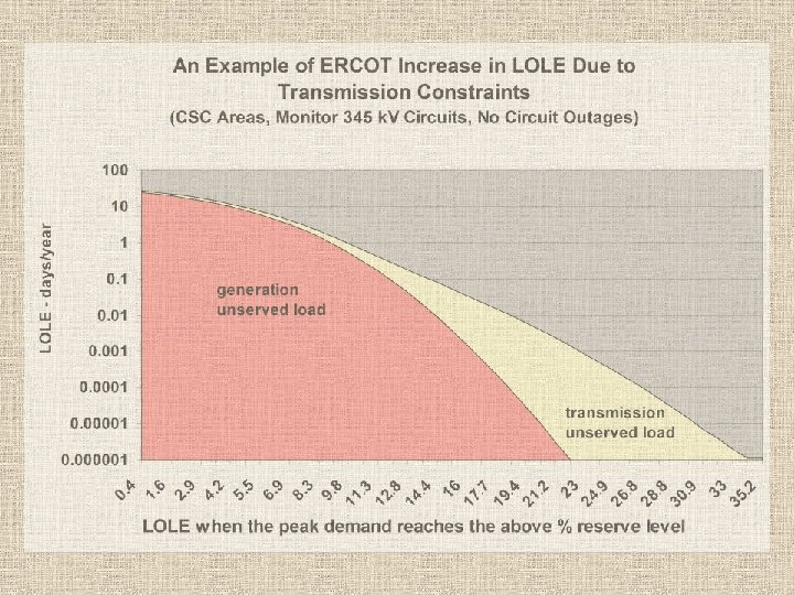
Load shedding to remove Austrop-Sandow circuit overloads generation LOLE RESV% 22. 1 21. 2 20. 3 19. 4 18. 5 17. 7 16. 9 16. 0 15. 2 14. 4 13. 6 12. 8 12. 0 11. 3 10. 5 9. 8 9. 1 8. 3 7. 6 6. 9 6. 2 5. 5 4. 9 4. 2 3. 5 2. 9 2. 2 1. 6 1. 0 0. 4 LOAD-MW 66956. 00 67456. 00 67956. 00 68456. 00 68956. 00 69456. 00 69956. 00 70456. 00 70956. 00 71456. 00 71956. 00 72456. 00 72956. 00 73456. 00 73956. 00 74456. 00 74956. 00 75456. 00 75956. 00 76456. 00 76956. 00 77456. 00 77956. 00 78456. 00 78956. 00 79456. 00 79956. 00 80456. 00 80956. 00 81456. 00 LOLP 0. 0000004 0. 0000012 0. 0000039 0. 0000115 0. 0000328 0. 0000894 0. 0002330 0. 0005806 0. 0013812 0. 0031339 0. 0067733 0. 0139248 0. 0271876 0. 0503270 0. 0881587 0. 1458544 0. 2274701 0. 3338294 0. 4604444 0. 5966979 0. 7275037 0. 8376617 0. 9172952 0. 9653328 0. 9886289 0. 9972702 0. 9995617 0. 9999568 0. 9999959 0. 9999987 TLOP 0. 0000001 0. 0000002 0. 0000004 0. 0000006 0. 0000010 0. 0000015 0. 0000024 0. 0000036 0. 0000055 0. 0000082 0. 0000120 0. 0000173 0. 0000246 0. 0000345 0. 0000472 0. 0000641 0. 0000847 0. 0001094 0. 0001386 0. 0001670 0. 0001914 0. 0002067 0. 0002070 0. 0001889 0. 0001498 0. 0001027 0. 0000594 0. 0000280 0. 0000104 GLOL-D/Y 0. 000001 0. 000003 0. 000010 0. 000029 0. 000084 0. 000232 0. 000615 0. 001563 0. 003799 0. 008833 0. 019635 0. 041690 0. 084488 0. 163376 0. 301211 0. 529378 0. 886719 1. 416075 2. 158461 3. 146670 4. 400033 5. 922297 7. 703882 9. 723858 11. 947046 14. 317933 16. 754972 19. 161745 21. 463148 23. 621519 transmission LOLE TLOL-D/Y 0. 000000 0. 000001 0. 000002 0. 000003 0. 000004 0. 000007 0. 000011 0. 000017 0. 000027 0. 000041 0. 000062 0. 000092 0. 000135 0. 000195 0. 000277 0. 000390 0. 000539 0. 000733 0. 000982 0. 001284 0. 001641 0. 002040 0. 002472 0. 002903 0. 003325 0. 003700 0. 004023 0. 004293 0. 004478 TOTL-D/Y 0. 000001 0. 000004 0. 000011 0. 000031 0. 000086 0. 000236 0. 000622 0. 001574 0. 003816 0. 008860 0. 019676 0. 041752 0. 084580 0. 163511 0. 301406 0. 529655 0. 887109 1. 416615 2. 159193 3. 147652 4. 401317 5. 923937 7. 705923 9. 726330 11. 949949 14. 321258 16. 758673 19. 165768 21. 467442 23. 625998

Overall effect of removing all transmission overloads on the LOLE Pr [gen is in service] 1 single area unserved load additional unserved load due to a transmission constraint 0 0 x MW load
![Pr [gen is out of service] Overall effect of removing all transmission overloads on](https://present5.com/presentation/40593ed57d0acbe5f2166afb9c88becf/image-69.jpg "Pr [gen is out of service] Overall effect of removing all transmission overloads on")
Pr [gen is out of service] Overall effect of removing all transmission overloads on the LOLE 1 0 Generation Capability additional unserved load due to a transmission constraint single area unserved load MW increasing load 0

See my dissertation on egpreston. com for more details. The End
40593ed57d0acbe5f2166afb9c88becf.ppt