Gene Structure Gene Finding Part II David

Gene Structure & Gene Finding: Part II David Wishart david. wishart@ualberta. ca

Contacting Me… • 200 emails a day – not the best way to get an instant response • Subject line: Bioinf 301 or Bioinf 501 • Preferred method… – Talk to me after class – Talk to me before class – Ask questions in class – Visit my office after 4 pm (Mon. – Fri. ) – Contact my bioinformatics assistant – Dr. An Chi Guo (anchiguo@gmail. com)

Lecture Notes Available At: • http: //www. wishartlab. com/ • Go to the menu at the top of the page, look under Courses

Outline for Next 3 Weeks • • Genes and Gene Finding (Prokaryotes) Genes and Gene Finding (Eukaryotes) Genome and Proteome Annotation Fundamentals of Transcript Measurement • Introduction to Microarrays • More details on Microarrays

Assignment Schedule • Gene finding - genome annotation – (Assigned Oct. 31, due Nov. 7) • Microarray analysis – (Assigned Nov. 7, due Nov. 19) • Protein structure analysis – (Assigned Nov. 21, due Nov. 28) Each assignment is worth 5% of total grade, 10% off for each day late

Objectives* • Learn key features of eukaryotic gene structure and transcript processing • Learn/memorize a few key eukaryotic gene signature sequences • Learn about RNA c. DNA preparation • Review algorithms and web tools for eukaryotic gene identification • Measuring/assessing gene prediction (limitations, methods)

23, 000 metabolite

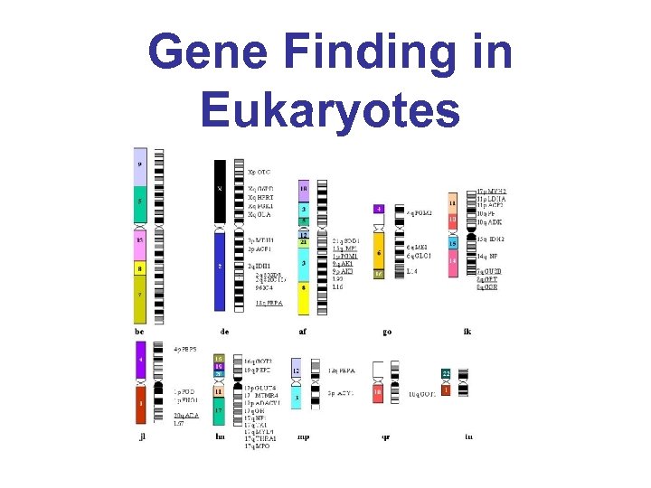Gene Finding in Eukaryotes

Eukaryotes* • • Complex gene structure Large genomes (0. 1 to 10 billion bp) Exons and Introns (interrupted) Low coding density (<30%) – 3% in humans, 25% in Fugu, 60% in yeast • Alternate splicing (40 -60% of all genes) • High abundance of repeat sequence (50% in humans) and pseudo genes • Nested genes: overlapping on same or opposite strand or inside an intron

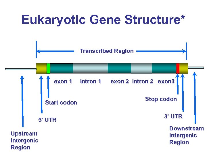Eukaryotic Gene Structure* Transcribed Region exon 1 Start codon 5’ UTR Upstream Intergenic Region intron 1 exon 2 intron 2 exon 3 Stop codon 3’ UTR Downstream Intergenic Region

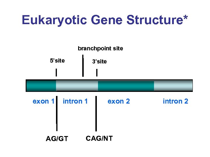Eukaryotic Gene Structure* branchpoint site 5’site exon 1 3’site intron 1 AG/GT exon 2 CAG/NT intron 2

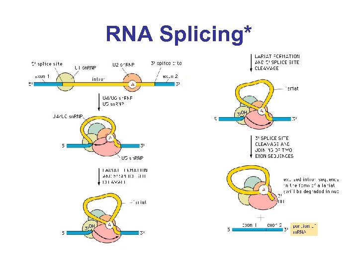RNA Splicing*

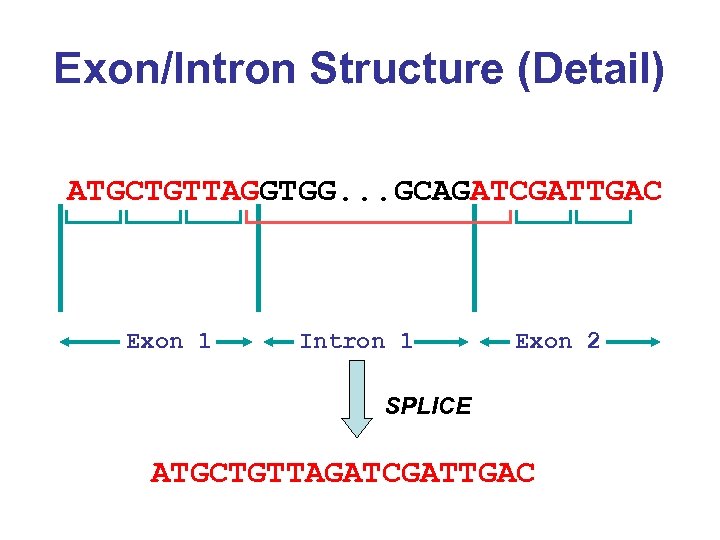Exon/Intron Structure (Detail) ATGCTGTTAGGTGG. . . GCAGATCGATTGAC Exon 1 Intron 1 Exon 2 SPLICE ATGCTGTTAGATCGATTGAC

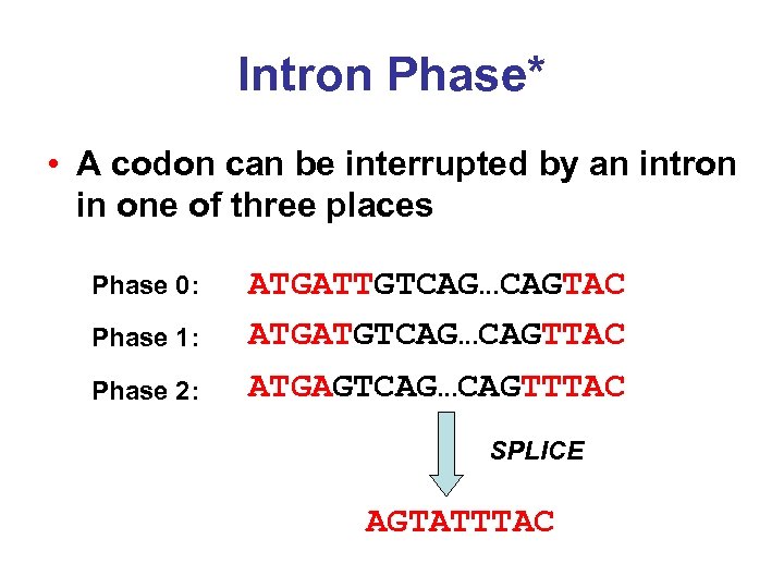Intron Phase* • A codon can be interrupted by an intron in one of three places Phase 0: Phase 1: Phase 2: ATGATTGTCAG…CAGTAC ATGATGTCAG…CAGTTAC ATGAGTCAG…CAGTTTAC SPLICE AGTATTTAC

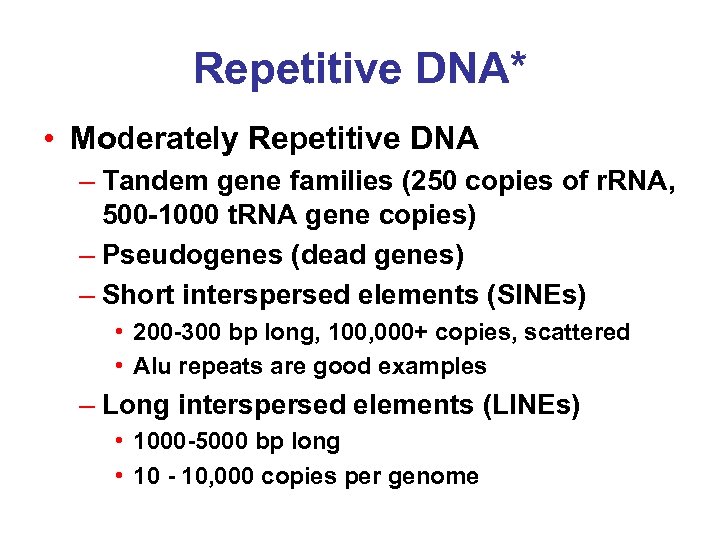Repetitive DNA* • Moderately Repetitive DNA – Tandem gene families (250 copies of r. RNA, 500 -1000 t. RNA gene copies) – Pseudogenes (dead genes) – Short interspersed elements (SINEs) • 200 -300 bp long, 100, 000+ copies, scattered • Alu repeats are good examples – Long interspersed elements (LINEs) • 1000 -5000 bp long • 10 - 10, 000 copies per genome

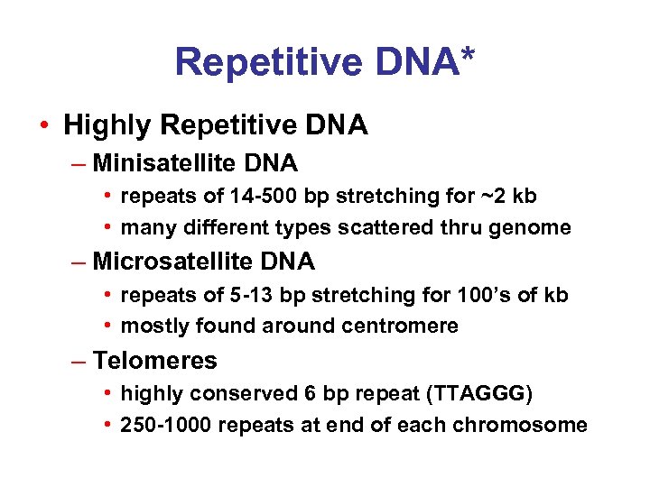Repetitive DNA* • Highly Repetitive DNA – Minisatellite DNA • repeats of 14 -500 bp stretching for ~2 kb • many different types scattered thru genome – Microsatellite DNA • repeats of 5 -13 bp stretching for 100’s of kb • mostly found around centromere – Telomeres • highly conserved 6 bp repeat (TTAGGG) • 250 -1000 repeats at end of each chromosome

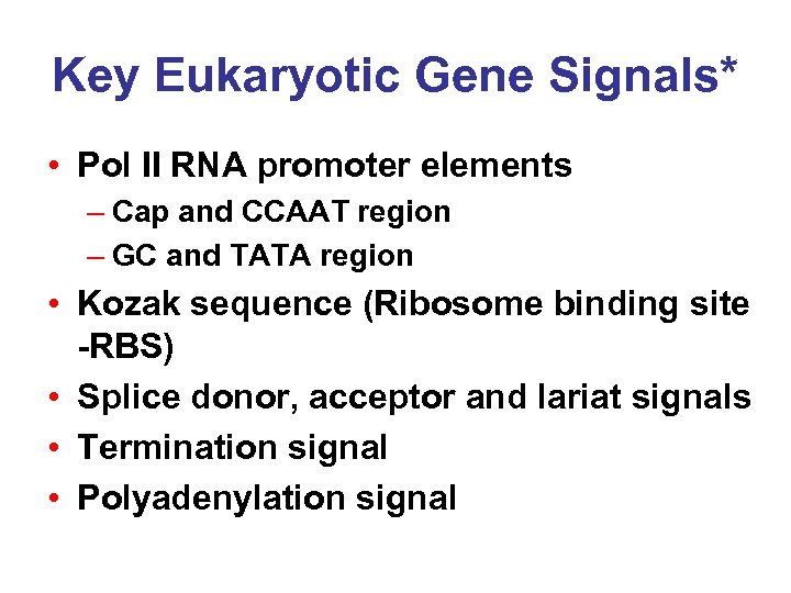Key Eukaryotic Gene Signals* • Pol II RNA promoter elements – Cap and CCAAT region – GC and TATA region • Kozak sequence (Ribosome binding site -RBS) • Splice donor, acceptor and lariat signals • Termination signal • Polyadenylation signal

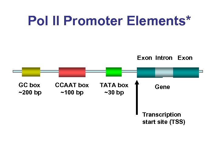Pol II Promoter Elements* Exon Intron Exon GC box ~200 bp CCAAT box ~100 bp TATA box ~30 bp Gene Transcription start site (TSS)

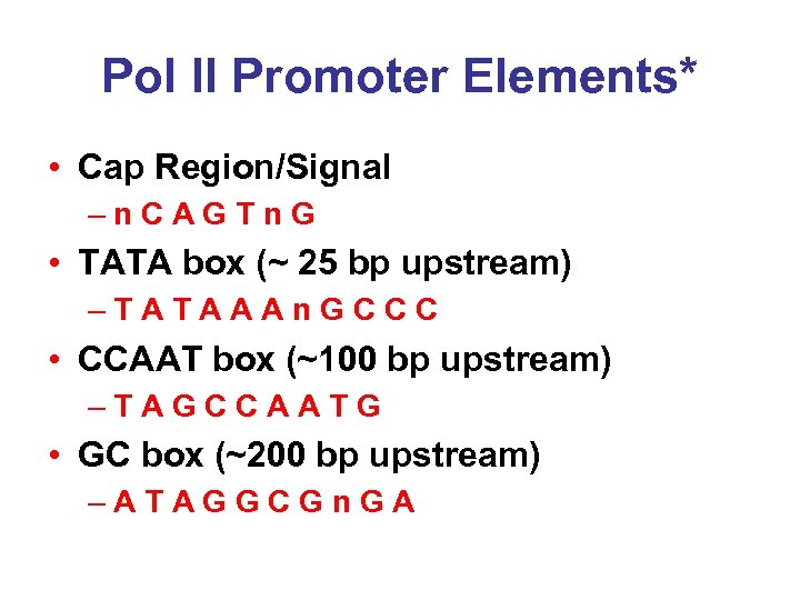Pol II Promoter Elements* • Cap Region/Signal –n. CAGTn. G • TATA box (~ 25 bp upstream) –TATAAAn. GCCC • CCAAT box (~100 bp upstream) –TAGCCAATG • GC box (~200 bp upstream) –ATAGGCGn. GA

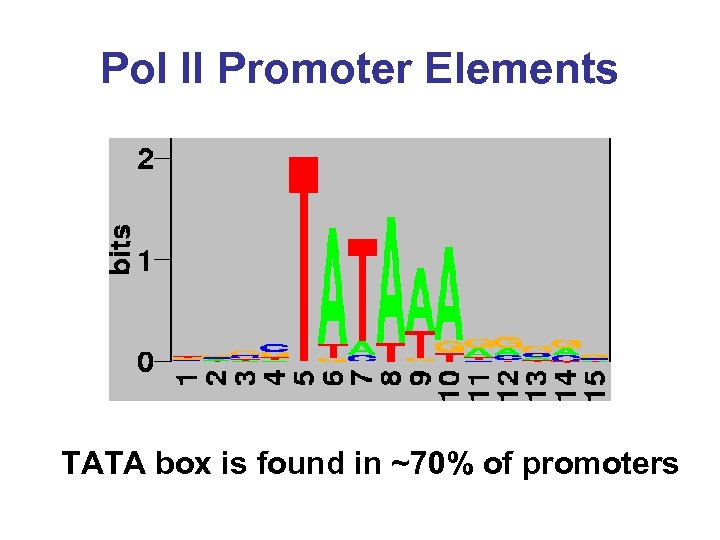Pol II Promoter Elements TATA box is found in ~70% of promoters

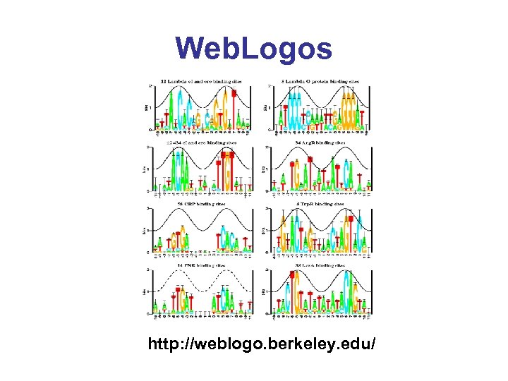Web. Logos http: //weblogo. berkeley. edu/

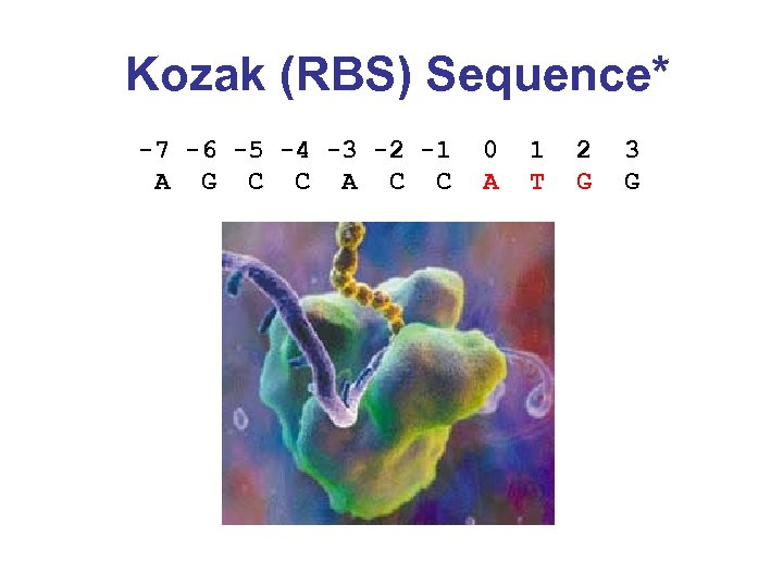Kozak (RBS) Sequence* -7 -6 -5 -4 -3 -2 -1 A G C C A C C 0 A 1 T 2 G 3 G

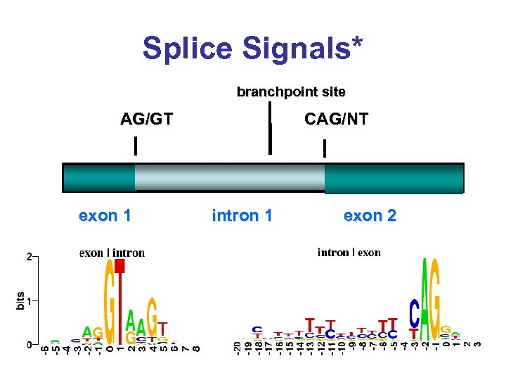Splice Signals* branchpoint site CAG/NT AG/GT exon 1 intron 1 exon 2

Splice Sites* • Not all splice sites are real • ~0. 5% of splice sites are non-canonical (i. e. the intron is not GT. . . AG) • It is estimated that 5% of human genes may have non-canonical splice sites • ~50% of higher eukaryotes are alternately spliced (different exons are brought together)

Miscellaneous Signals* • Polyadenylation signal – A A T A A A or A T T A A A – Located 20 bp upstream of poly-A cleavage site • Termination Signal –AGTGTTCA – Located ~30 bp downstream of poly-A cleavage site

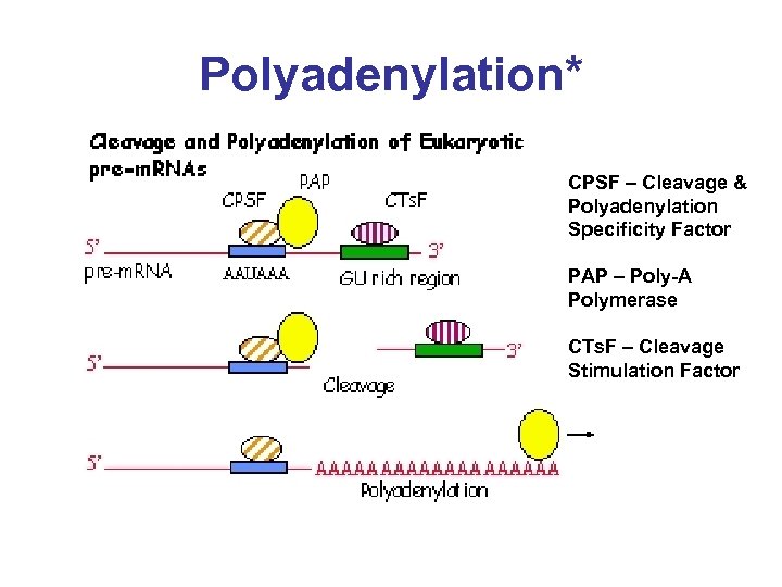Polyadenylation* CPSF – Cleavage & Polyadenylation Specificity Factor PAP – Poly-A Polymerase CTs. F – Cleavage Stimulation Factor

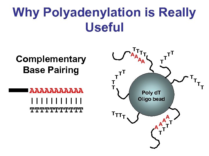Why Polyadenylation is Really Useful Complementary Base Pairing AAAAAA |||||| TTTTTT TT AA T T T TT TT T Poly d. T Oligo bead T A A TT T T

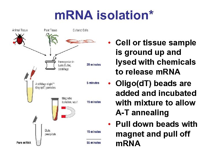m. RNA isolation* • • Cell or tissue sample is ground up and lysed with chemicals to release m. RNA • Oligo(d. T) beads are added and incubated with mixture to allow A-T annealing • Pull down beads with magnet and pull off m. RNA

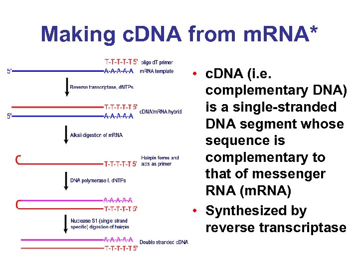Making c. DNA from m. RNA* • c. DNA (i. e. complementary DNA) is a single-stranded DNA segment whose sequence is complementary to that of messenger RNA (m. RNA) • Synthesized by reverse transcriptase

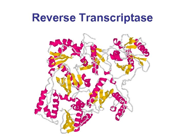Reverse Transcriptase

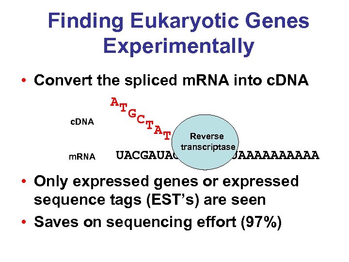Finding Eukaryotic Genes Experimentally • Convert the spliced m. RNA into c. DNA AT c. DNA m. RNA GC TA Reverse T CTGTACTA transcriptase UACGAUAGACAUGAUAAAAA • Only expressed genes or expressed sequence tags (EST’s) are seen • Saves on sequencing effort (97%)

Finding Eukaryotic Genes Computationally* • Content-based Methods – GC content, hexamer repeats, composition statistics, codon frequencies • Site-based Methods – donor sites, acceptor sites, promoter sites, start/stop codons, poly. A signals, lengths • Comparative Methods – sequence homology, EST searches • Combined Methods

Content-Based Methods* • Cp. G islands – High GC content in 5’ ends of genes • Codon Bias – Some codons are strongly preferred in coding regions, others are not • Positional Bias – 3 rd base tends to be G/C rich in coding regions • Ficketts Method – looks for unequal base composition in different clusters of i, i+3, i+6 bases - Test. Code graph

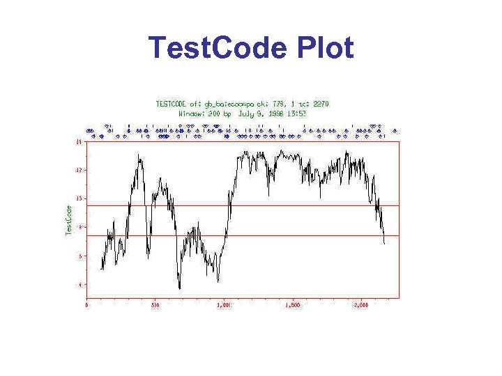Test. Code Plot

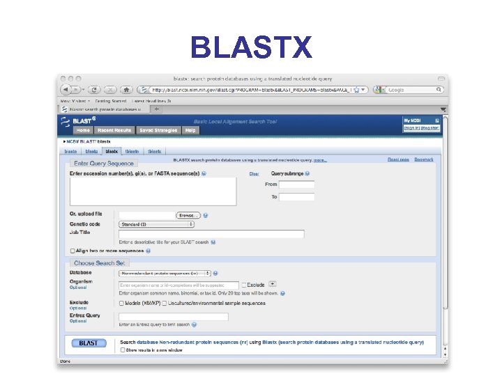
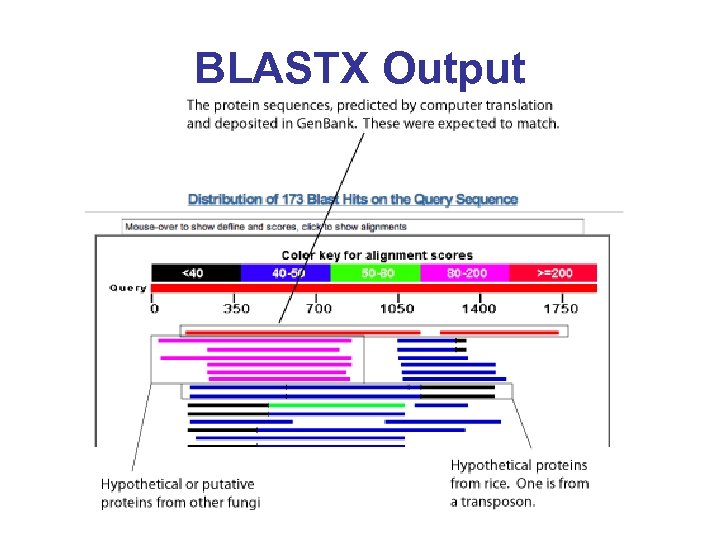
Comparative Methods* • Do a BLASTX search of all 6 reading frames against known proteins in Gen. Bank • Assumes that the organism under study has genes that are homologous to known genes (used to be a problem, in 2001 analysis of chr. 22 only 50% of genes were similar to known proteins) • BLAST against EST database (finds possible or probable 3’ end of c. DNAs)

BLASTX

BLASTX Output

Site-Based Methods* • Based on identifying gene signals (promoter elements, splice sites, start/stop codons, poly. A sites, etc. ) • Wide range of methods – consensus sequences – weight matrices – neural networks – decision trees – hidden markov models (HMMs)

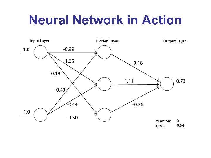
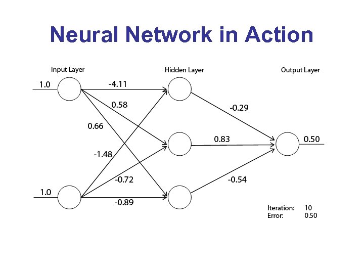
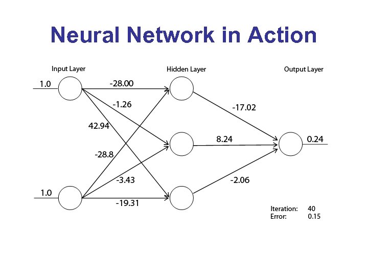
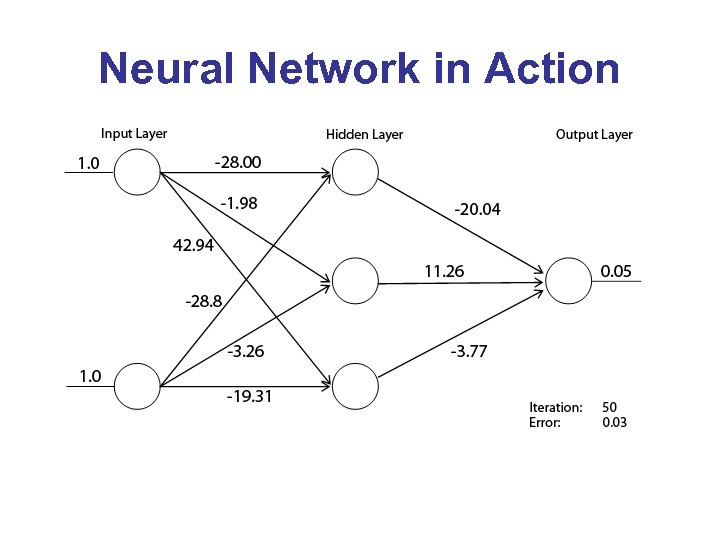
Neural Networks • Automated method for classification or pattern recognition • First described in detail in 1986 • Mimic the way the brain works • Use Matrix Algebra in calculations • Require “training” on validated data • Garbage in = Garbage out

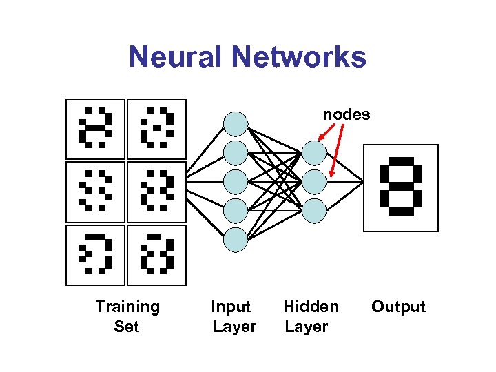Neural Networks nodes Training Set Input Layer Hidden Layer Output

Neural Network Applications • • Used in Intron/Exon Finding Used in Secondary Structure Prediction Used in Membrane Helix Prediction Used in Phosphorylation Site Prediction Used in Glycosylation Site Prediction Used in Splice Site Prediction Used in Signal Peptide Recognition

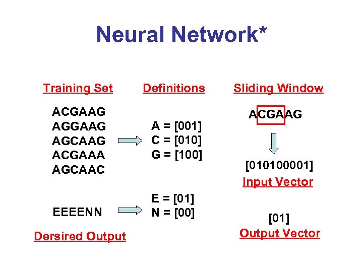Neural Network* Training Set ACGAAG AGCAAG ACGAAA AGCAAC EEEENN Dersired Output Definitions A = [001] C = [010] G = [100] E = [01] N = [00] Sliding Window ACGAAG [010100001] Input Vector [01] Output Vector

Neural Network Training* 1 [010100001] ACGAAG Input Vector . 2. 4. 1. 1. 0. 4. 7. 1. 1. 0. 0. 0 [. 6. 4. 6]. 2. 4. 1. 0. 3. 5. 1. 1. 0. 5. 3. 1 Weight Matrix 1 1 - e-x. 1. 8. 0. 2. 3. 3 [. 24. 74] compare [0 1] Hidden Weight Output Layer Matrix 2 Vector

Back Propagation* 1 [010100001] Input Vector . 2. 4. 1 1 - e-x. 1. 0. 4. 02. 83. 7. 1. 1. 1. 8. 0. 1. 1. 0. 0. 0 [. 6. 4. 6]. 0. 2. 23 [. 24. 74]. 3. 3. 2. 4. 1 compare. 22. 33. 0. 3. 5. 1. 1. 0 [0 1]. 5. 3. 1 Weight Matrix 1 Hidden Weight Output Layer Matrix 2 Vector

Calculate New Output* 1 [010100001] Input Vector . 1. 1. 1. 2. 0. 4. 7. 1. 1. 0. 0. 0 [. 7. 4. 7]. 2. 2. 1. 0. 3. 5. 1. 3. 0. 5. 3. 3 Weight Matrix 1 1 - e-x. 02. 83. 00. 23. 22. 33 [. 16. 91] Converged! [0 1] Hidden Weight Output Layer Matrix 2 Vector

Train on Second Input Vector* 1 [100001001] ACGAAG Input Vector . 1. 1. 1. 2. 0. 4. 7. 1. 1. 0. 0. 0 [. 8. 6. 5]. 2. 2. 1. 0. 3. 5. 1. 3. 0. 5. 3. 3 Weight Matrix 1 1 - e-x. 02. 83. 00. 23. 22. 33 [. 12. 95] Compare [0 1] Hidden Weight Output Layer Matrix 2 Vector

Back Propagation* 1 [010100001] Input Vector . 1. 1. 1 1 - e-x. 2. 0. 4. 01. 84. 7. 1. 1. 02. 83. 0. 1. 1. 24. 0. 0. 0 [. 8. 6. 5]. 00. 23 [. 12. 95]. 22. 33. 2. 2. 1 compare. 21. 34. 0. 3. 5. 1. 3. 0 [0 1]. 5. 3. 3 Weight Matrix 1 Hidden Weight Output Layer Matrix 2 Vector

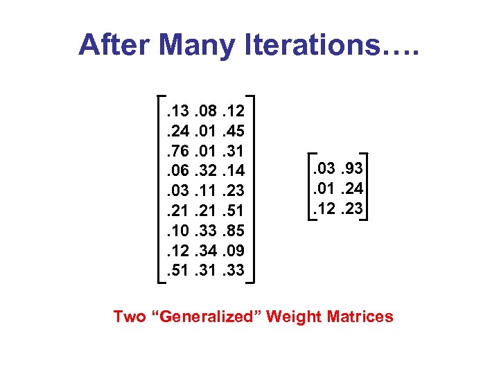After Many Iterations…. . 13. 08. 12. 24. 01. 45. 76. 01. 31. 06. 32. 14. 03. 11. 23. 21. 51. 10. 33. 85. 12. 34. 09. 51. 33 . 03. 93. 01. 24. 12. 23 Two “Generalized” Weight Matrices

Neural Network in Action

Neural Network in Action

Neural Network in Action

Neural Network in Action

Neural Network in Action

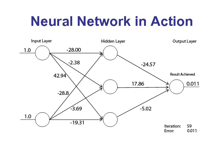Neural Network in Action

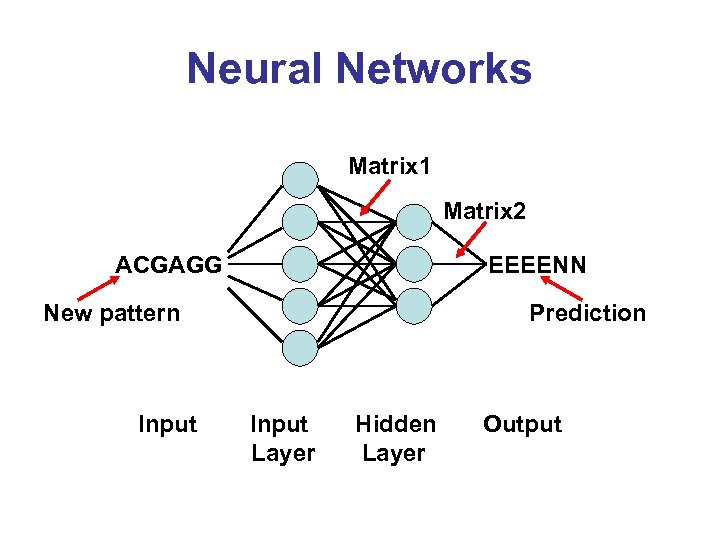Neural Networks Matrix 1 Matrix 2 ACGAGG EEEENN New pattern Input Prediction Input Layer Hidden Layer Output

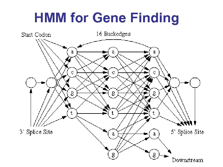HMM for Gene Finding

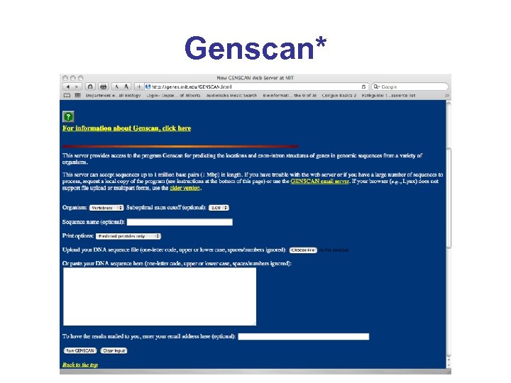
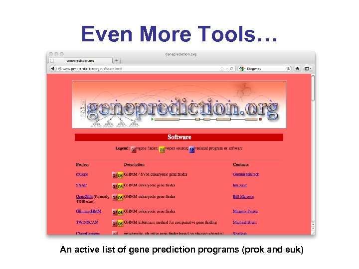
Combined Methods • Bring 2 or more methods together (usually site detection + composition) • Grail. EXP (http: //compbio. ornl. gov/Grail-1. 3/) • Gene. Mark-E (http: //exon. biology. gatech. edu/) • HMMgene (http: //www. cbs. dtu. dk/services/HMMgene/) • GENSCAN(http: //genes. mit. edu/GENSCAN. html) • GRPL (Gene. Tool/Bio. Tools)

Genscan*

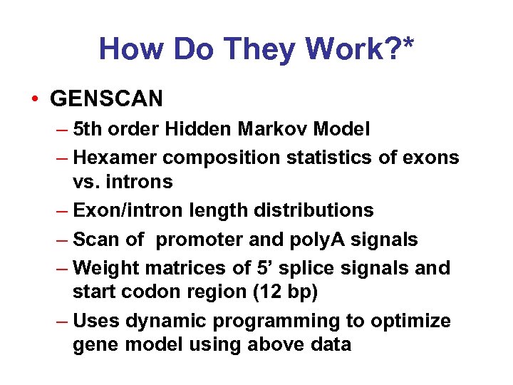How Do They Work? * • GENSCAN – 5 th order Hidden Markov Model – Hexamer composition statistics of exons vs. introns – Exon/intron length distributions – Scan of promoter and poly. A signals – Weight matrices of 5’ splice signals and start codon region (12 bp) – Uses dynamic programming to optimize gene model using above data

Correlation (x 100) How Well Do They Do? Method Burset & Guigio test set (1996)

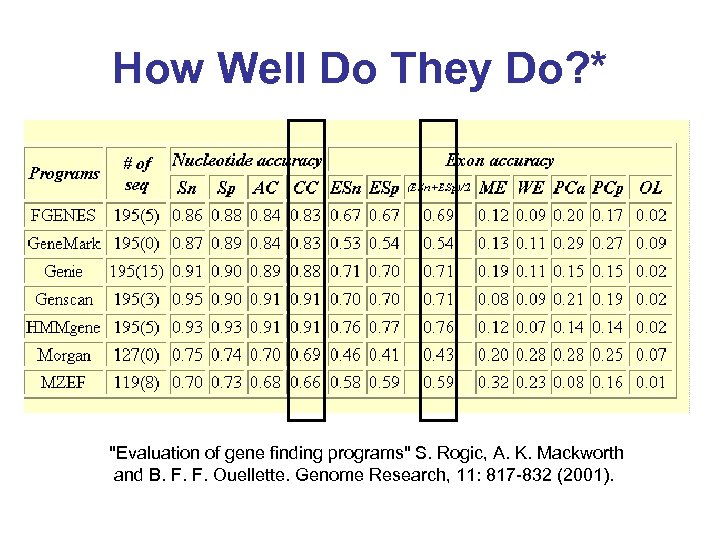How Well Do They Do? * "Evaluation of gene finding programs" S. Rogic, A. K. Mackworth and B. F. F. Ouellette. Genome Research, 11: 817 -832 (2001).

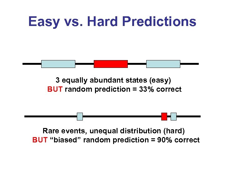Easy vs. Hard Predictions 3 equally abundant states (easy) BUT random prediction = 33% correct Rare events, unequal distribution (hard) BUT “biased” random prediction = 90% correct

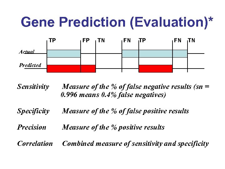Gene Prediction (Evaluation)* TP FP TN FN TP FN TN Actual Predicted Sensitivity Measure of the % of false negative results (sn = 0. 996 means 0. 4% false negatives) Specificity Measure of the % of false positive results Precision Measure of the % positive results Correlation Combined measure of sensitivity and specificity

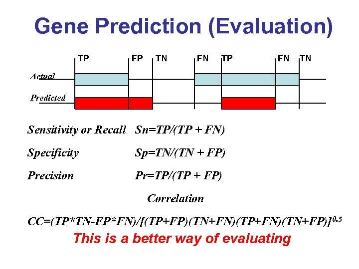Gene Prediction (Evaluation) TP FP TN FN TP FN TN Actual Predicted Sensitivity or Recall Sn=TP/(TP + FN) Specificity Sp=TN/(TN + FP) Precision Pr=TP/(TP + FP) Correlation CC=(TP*TN-FP*FN)/[(TP+FP)(TN+FN)(TP+FN)(TN+FP)]0. 5 This is a better way of evaluating

Different Strokes for Different Folks • Precision and specificity statistics favor conservative predictors that make no prediction when there is doubt about the correctness of a prediction, while the sensitivity (recall) statistic favors liberal predictors that make a prediction if there is a chance of success. • Information retrieval papers report precision and recall, while bioinformatics papers tend to report specificity and sensitivity.

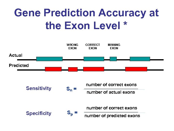Gene Prediction Accuracy at the Exon Level * WRONG EXON CORRECT EXON MISSING EXON Actual Predicted Sensitivity Specificity Sn = Sp = number of correct exons number of actual exons number of correct exons number of predicted exons

Better Approaches Are Emerging. . . • Programs that combine site, comparative and composition (3 in 1) – Genome. Scan, FGENESH++, Twinscan • Programs that use synteny between organisms – ROSETTA, SLAM, SGP • Programs that combine predictions from multiple predictors – Gene. Comber, Augustus

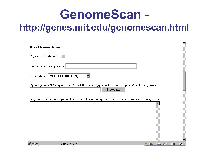Genome. Scan http: //genes. mit. edu/genomescan. html

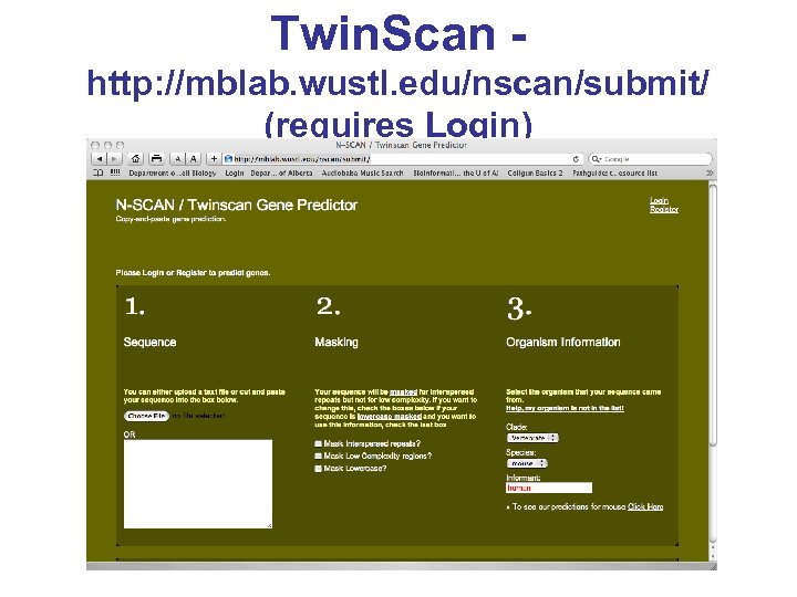Twin. Scan http: //mblab. wustl. edu/nscan/submit/ (requires Login)

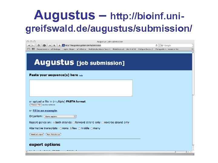Augustus – http: //bioinf. unigreifswald. de/augustus/submission/

Even More Tools… An active list of gene prediction programs (prok and euk)

Gene Finding with Gen. Scan & Company • Go to your preferred website • Paste in the DNA sequence of your favorite EUKARYOTIC genome (this won’t work for prokaryotic genomes and it won’t necessarily work for viral or phage genomes) • Press the submit button • Output will typically be presented in a new screen or emailed to you

Outstanding Issues* • Most Gene finders don’t handle UTRs (untranslated regions) • ~40% of human genes have non-coding 1 st exons (UTRs) • Most gene finders don’t’ handle alternative splicing • Most gene finders don’t handle overlapping or nested genes • Most can’t find non-protein genes (t. RNAs)

Bottom Line. . . • Gene finding in eukaryotes is not yet a “solved” problem • Accuracy of the best methods approaches 80% at the exon level (90% at the nucleotide level) in coding-rich regions (much lower for whole genomes) • Gene predictions should always be verified by other means (c. DNA sequencing, BLAST search, Mass spec. ) • Homework: Try testing some of the web servers I have mentioned today

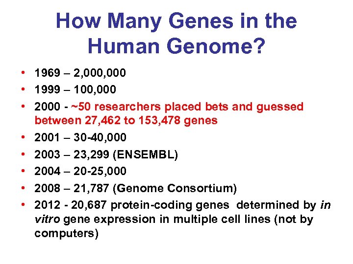How Many Genes in the Human Genome? • 1969 – 2, 000 • 1999 – 100, 000 • 2000 - ~50 researchers placed bets and guessed between 27, 462 to 153, 478 genes • 2001 – 30 -40, 000 • 2003 – 23, 299 (ENSEMBL) • 2004 – 20 -25, 000 • 2008 – 21, 787 (Genome Consortium) • 2012 - 20, 687 protein-coding genes determined by in vitro gene expression in multiple cell lines (not by computers)