Gaussian Processes for Statistical Soil Modeling of the

Gaussian Processes for Statistical Soil Modeling of the Tropics CMU/Tech. Bridge. World: Juan Pablo Gonzalez Drew Bagnell CIAT Team: Simon Cook, Thomas Oberthur, Andrew Jarvis, Mauricio Rincon

Introduction: What is CIAT? n International Center for Tropical Agriculture q q Is a not-for-profit organization Conducts socially and environmentally progressive research in developing countries aimed at n reducing hunger and poverty n preserving natural resources Works through partnerships with farmers, scientists, and policy makers 800 people, 120 researchers from 37 different countries 2

Introduction: CIAT locations n One of 15 future harvest centers in q q n Cali, Colombia (headquarters) Kampala, Uganda (African Regional Office) Vientiane, Lao (Asian Regional Office) Honduras, Ecuador, Nicaragua, Bolivia, Kenya, Brazil, Sri Lanka and Thailand, amongst others. Funded by CGIAR q q Consultative Group on International Agricultural Research 58 countries, private foundations, and international organizations CGIAR Members: World Bank, FAO, Ford Foundation, Rockefeller Foundation, Kellog Foundation, USA, Canada, U. K. , Australia, New Zealand, Sweden, Portugal, Norway, Denmark, Austria, Italy, India, Pakistan, Kenya, Nigeria, Bangladesh, Belgium, Brazil, China, Colombia, Cote d'Ivoire, Egypt, Finland, France, Germany, Indonesia, Iran, Ireland, Israel, Japan, Korea, Luxembourg, Malaysia, Mexico, Morocco, The Netherlands, Peru, The Philippines, Portugal, Republic of South Africa, Romania, Russian Federation, Spain, Switzerland, Syrian, Arab Republic, Thailand, Turkey, Uganda 3

Introduction: What is Tech. Bridge. World? n n An initiative within Carnegie Mellon University Mission: q n To collaboratively design and implement creative technological solutions that will benefit developing communities around the world “To bridge the world with technology” 5

Introduction: Task at Hand n Input: q q q n Soil scientists from CIAT Computer Scientists from CMU/Tech. Bridge. World 2500 Field samples from Honduras Result: q Statistical Soil Modeling for The Tropics 6

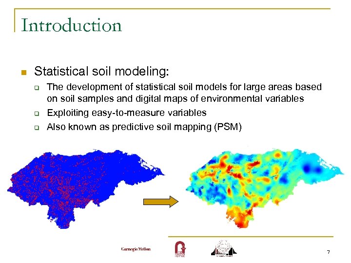Introduction n Statistical soil modeling: q q q The development of statistical soil models for large areas based on soil samples and digital maps of environmental variables Exploiting easy-to-measure variables Also known as predictive soil mapping (PSM) 7

Introduction n Importance q To detect opportunities n q q To reduce risk of failure in new crops To detect threats n q Target soil-sensitive crops confidently within new areas Assess impact of climate change To understand soil interactions with land use n n Understand local hydrology Make decisions about appropriate changes in land use 8

Introduction n Why in the tropics? q q q Most developing countries are located in the tropics Most funding for soil analysis and modeling does not go to the tropics The tropics have distinct climate patterns from the rest of the globe n n n Only dry/wet season (instead of four seasons) Almost constant day length Main determinant factor for temperature is elevation 9

Introduction: Current Soil Map Coverage Throughout the World n Detailed soil maps: q q n USA: complete coverage at 1: 24, 000 – very extensive and expensive (~30 m grid size) 68% of the countries (31% by area) have complete coverage at 1: 1, 000 or better (1 km grid size) Rest of the World q 69% by area q FAO World Map 10

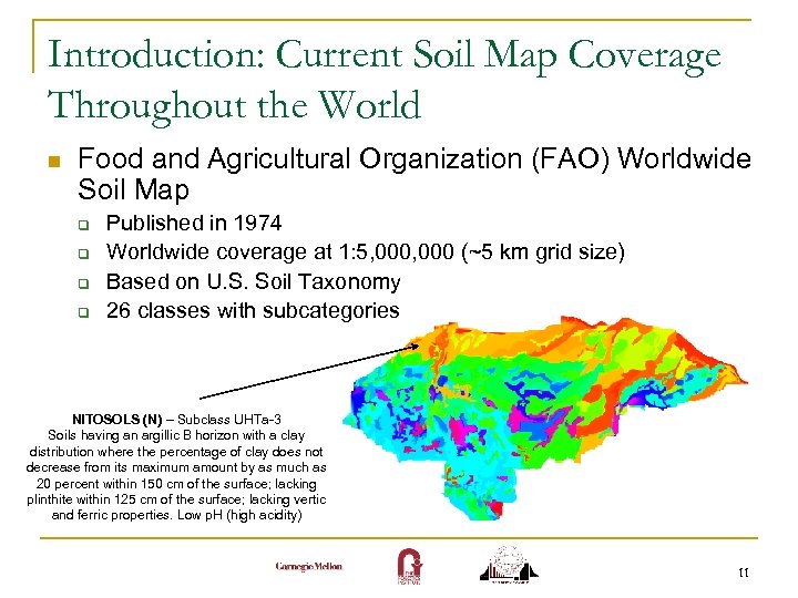Introduction: Current Soil Map Coverage Throughout the World n Food and Agricultural Organization (FAO) Worldwide Soil Map q q Published in 1974 Worldwide coverage at 1: 5, 000 (~5 km grid size) Based on U. S. Soil Taxonomy 26 classes with subcategories NITOSOLS (N) – Subclass UHTa-3 Soils having an argillic B horizon with a clay distribution where the percentage of clay does not decrease from its maximum amount by as much as 20 percent within 150 cm of the surface; lacking plinthite within 125 cm of the surface; lacking vertic and ferric properties. Low p. H (high acidity) 11

Previous Work: FAO Soil Map n Problems: q q q Made with information and technology of 1960 n Significant changes in technologies such as GPS, remote sensing and GIS Categorical data n Most soil types explain only a small proportion of the actual variation of properties n Soil variation is continuous n Soil attributes do not cluster perfectly: a cut on the basis of one attribute may split the variance of another attribute near its peak Dependent on subjective expert opinion Dependent on soil classification used Low resolution 13

Traditional Soil Survey n Three steps: q q q n Observation and measurement of ancillary data and soil profile Observations incorporated into implicit conceptual model Apply conceptual model to predict soil variation in unobserved sites Conceptual model uses factors of soil formation q Soil is a function of climate, topography, organisms, parent material, time (H. Jenny, 1941) 14

Predictive Soil Mapping (PSM) n Statistical model using factors of soil formation q n Soil is a function of climate, topography, organisms, parent material, time Goals q q q Exploit relationships between environmental variables and soil properties to improve data collection efficiency Produce and present data that better represent soil landscape continuity Explicitly incorporate expert knowledge in the design 15

PSM: Existing Approaches n Ordinary Kriging q q n Weighted local spatial averaging Spatial interpolation Does not use knowledge of soil materials or processes Requires a large number of closely-spaced samples Block Kriging, Indicator Kriging, Co-Kriging q q Extensions to include ancillary data Difficult to extend to more than one ancillary variable 16

PSM: Existing Approaches n Expert Systems q q n Use expert knowledge to establish rule-based relationships between environment and soil properties Do not use soil data to determine soil-landscape relationships Regression Trees q q Decision trees with linear models Promising – Good results in Australia (Henderson, 2004) 17

New Approach: Gaussian Processes n Generalization of Gaussian distribution to function space of infinite dimension q q q n n Probabilistic (Bayesian) model Completely determined by mean and covariance function Prediction with mean and variance (confidence intervals) Non-parametric Very powerful Complexity of model increases with more data Not new. It started as kriging and has evolved as a replacement for supervised Neural Networks 18

Gaussian Processes n Interpolation technique equivalent to: q q Neural Network with infinite number of hidden units Radial Basis functions, with infinite number of basis functions Least squares SVMs Kernel Ridge Regression 20

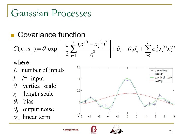Gaussian Processes n Covariance function 21

Available Data n n 2500 soil samples from Honduras Digital maps of Honduras with: q Climate: n n q Topography n q 90 -m elevation maps Vegetation Index n n Temperatures (max, min, average, etc) Precipitation (max, min, average, etc) Measurement of vegetation cover And derived variables 22

Gaussian Processes n Learning the hyperparameters q q q n Maximize the probability of the hyperparameters given the data Use scaled conjugate gradient descent Takes approximately 20 minutes with current data set Selecting variables q q Select most promising variables and incrementally add them to the model Would take 54 hrs for each variable selected! 23

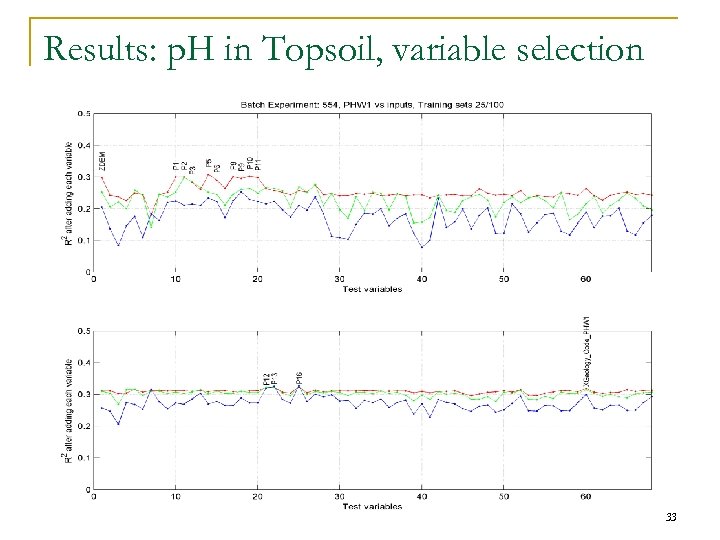
Gaussian Processes: Variable Selection n Greedy search on R 2 of validation set q q q Learn parameters for all variables @10% of training set Calculate R 2 on validation set for all variables @10% of training set Select variable with best R 2 Learn parameters @ 80% of training set with selected variables Calculate R 2 with selected variables @80% of training set Decide whether to continue based on R 2 on validation set for parameters R 2: coefficient of determination. Percentage of the variance explained by the model 24

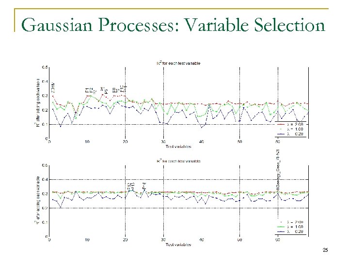Gaussian Processes: Variable Selection R 2: coefficient of determination. Percentage of the variance explained by the model 25

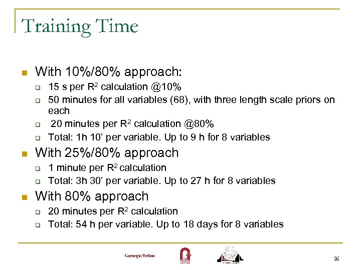Training Time n With 10%/80% approach: q q n With 25%/80% approach q q n 15 s per R 2 calculation @10% 50 minutes for all variables (68), with three length scale priors on each 20 minutes per R 2 calculation @80% Total: 1 h 10’ per variable. Up to 9 h for 8 variables 1 minute per R 2 calculation Total: 3 h 30’ per variable. Up to 27 h for 8 variables With 80% approach q q 20 minutes per R 2 calculation Total: 54 h per variable. Up to 18 days for 8 variables 26

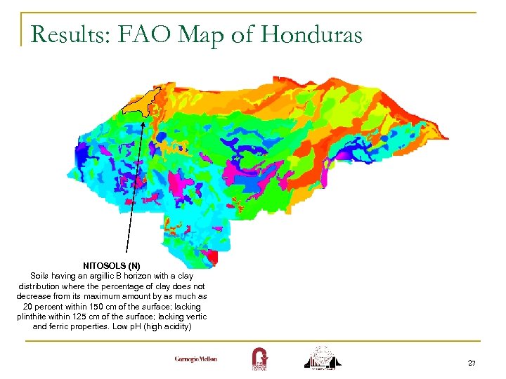Results: FAO Map of Honduras NITOSOLS (N) Soils having an argillic B horizon with a clay distribution where the percentage of clay does not decrease from its maximum amount by as much as 20 percent within 150 cm of the surface; lacking plinthite within 125 cm of the surface; lacking vertic and ferric properties. Low p. H (high acidity) 27

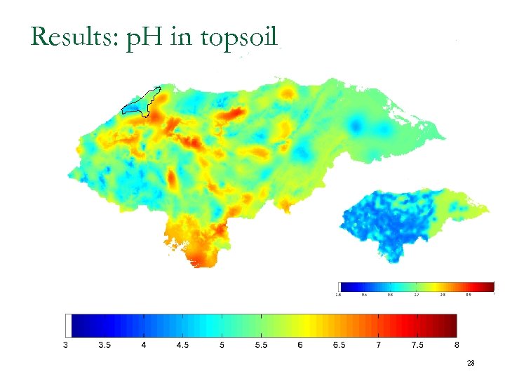Results: p. H in topsoil 28

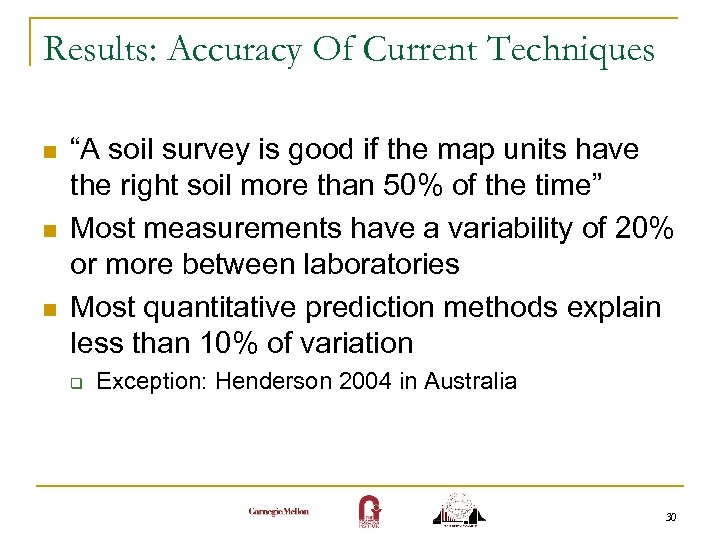Results: Accuracy Of Current Techniques n n n “A soil survey is good if the map units have the right soil more than 50% of the time” Most measurements have a variability of 20% or more between laboratories Most quantitative prediction methods explain less than 10% of variation q Exception: Henderson 2004 in Australia 30

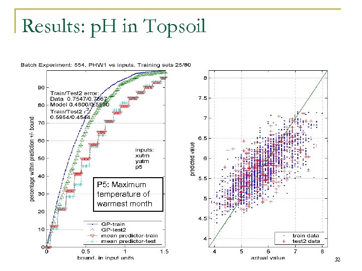
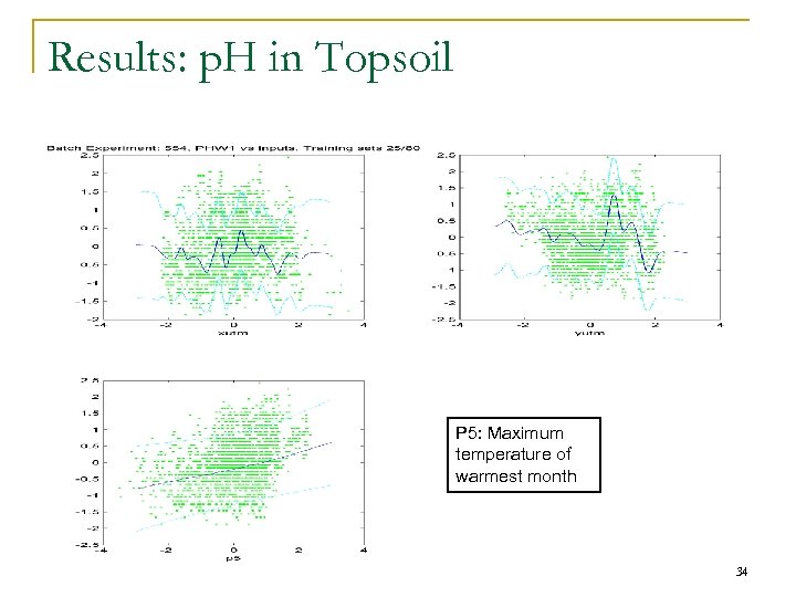
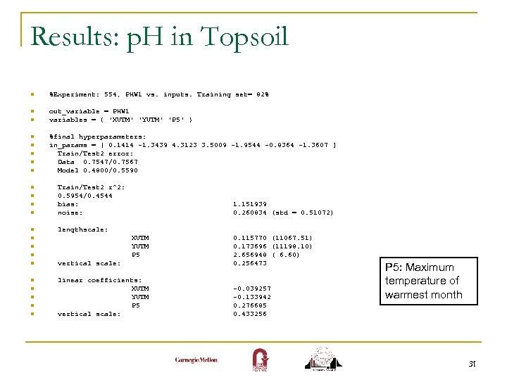Results: p. H in Topsoil n %Experiment: 554, PHW 1 vs. inputs. Training set= 82% n out_variable = PHW 1 variables = { 'XUTM' 'YUTM' 'P 5' } n n n %final hyperparameters: in_params = [ 0. 1414 -1. 3439 4. 3123 3. 5009 -1. 9544 -0. 8364 -1. 3607 ] Train/Test 2 error: Data 0. 7547/0. 7567 Model 0. 4800/0. 5590 n Train/Test 2 r^2: 0. 5954/0. 4544 bias: noise: n lengthscale: n n n 1. 151939 0. 260834 (std = 0. 51072) XUTM YUTM P 5 n vertical scale: 0. 115770 (11067. 51) 0. 173696 (11198. 10) 2. 656948 ( 6. 60) 0. 256473 n linear coefficients: XUTM YUTM P 5 vertical scale: -0. 039257 -0. 133942 0. 276685 0. 433256 n n n n P 5: Maximum temperature of warmest month 31

Results: p. H in Topsoil P 5: Maximum temperature of warmest month 32

Results: p. H in Topsoil, variable selection 33

Results: p. H in Topsoil P 5: Maximum temperature of warmest month 34

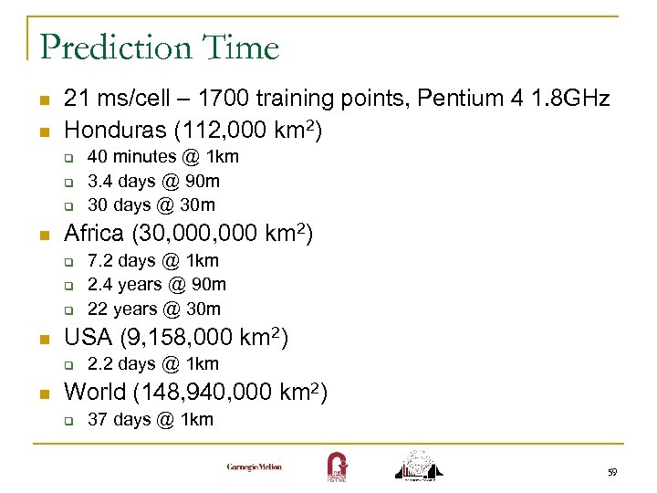Prediction Time n n 21 ms/cell – 1700 training points, Pentium 4 1. 8 GHz Honduras (112, 000 km 2) q q q n Africa (30, 000 km 2) q q q n 7. 2 days @ 1 km 2. 4 years @ 90 m 22 years @ 30 m USA (9, 158, 000 km 2) q n 40 minutes @ 1 km 3. 4 days @ 90 m 30 days @ 30 m 2. 2 days @ 1 km World (148, 940, 000 km 2) q 37 days @ 1 km 59

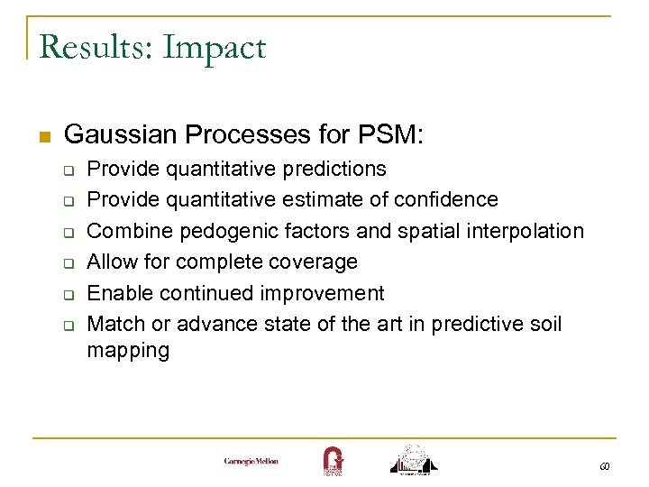Results: Impact n Gaussian Processes for PSM: q q q Provide quantitative predictions Provide quantitative estimate of confidence Combine pedogenic factors and spatial interpolation Allow for complete coverage Enable continued improvement Match or advance state of the art in predictive soil mapping 60

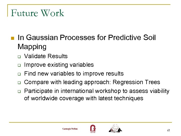Future Work n In Gaussian Processes for Predictive Soil Mapping q q q Validate Results Improve existing variables Find new variables to improve results Compare with leading approach: Regression Trees Participate in international workshop to assess viability of worldwide coverage with latest techniques 61

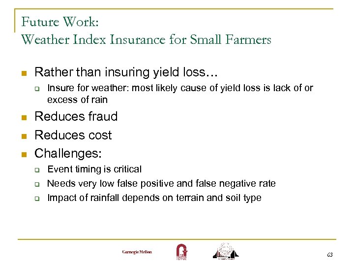Future Work: Weather Index Insurance for Small Farmers n Rather than insuring yield loss… q n n n Insure for weather: most likely cause of yield loss is lack of or excess of rain Reduces fraud Reduces cost Challenges: q q q Event timing is critical Needs very low false positive and false negative rate Impact of rainfall depends on terrain and soil type 63

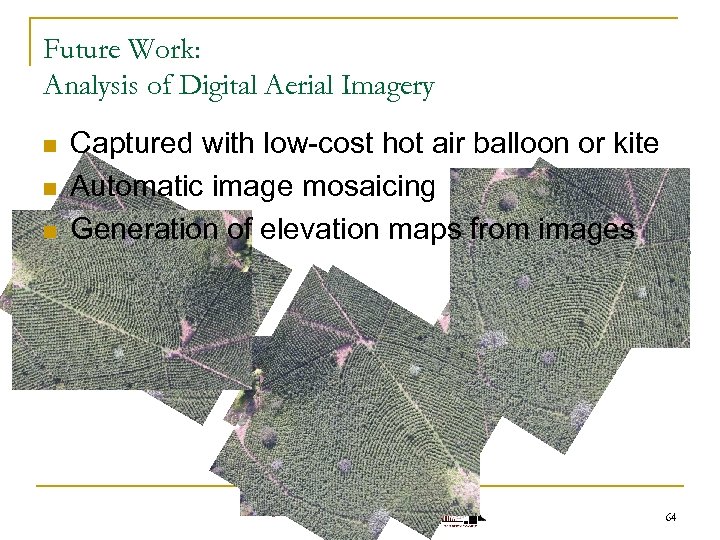Future Work: Analysis of Digital Aerial Imagery n n n Captured with low-cost hot air balloon or kite Automatic image mosaicing Generation of elevation maps from images 64

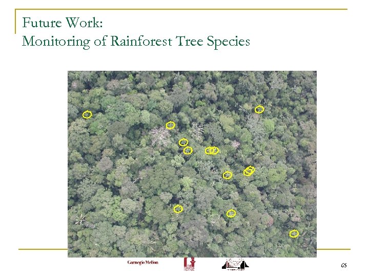Future Work: Monitoring of Rainforest Tree Species 65

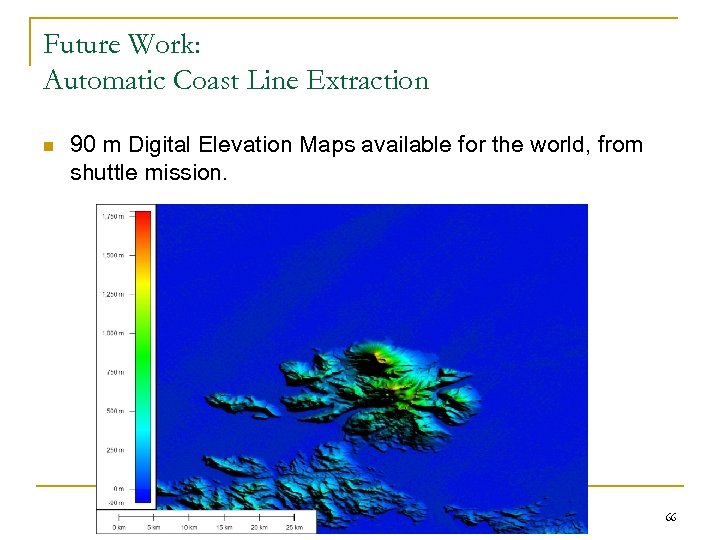Future Work: Automatic Coast Line Extraction n 90 m Digital Elevation Maps available for the world, from shuttle mission. 66

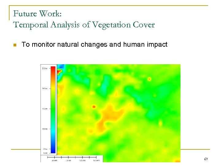Future Work: Temporal Analysis of Vegetation Cover n To monitor natural changes and human impact 67

Conclusions n Great contributions can be made by applying computer science techniques to other fields q n Scientists in other fields are frequently limited to off-the -shelf solutions Working with existing groups in developing countries can maximize impact of short-term work 68