0007804a8c3edd045bd7ebed8417f385.ppt
- Количество слайдов: 40

g. Store: Answering SPARQL Queries Via Subgraph Matching Lei Zou 1, Jinghui Mo 1, Lei Chen 2, M. Tamer Özsu 3, Dongyan Zhao 1 1 Peking University, 2 Hong Kong University of Science and Technology, 3 University of Waterloo 1
Outline • Background & Related Work • Overview of g. Store • Encoding Technique • VS*-tree & Query Algorithm • Experiments • Conclusions 2
Outline • Background & Related Work • Overview of g. Store • Encoding Technique • VS*-tree & Query Algorithm • Experiments • Conclusions 3
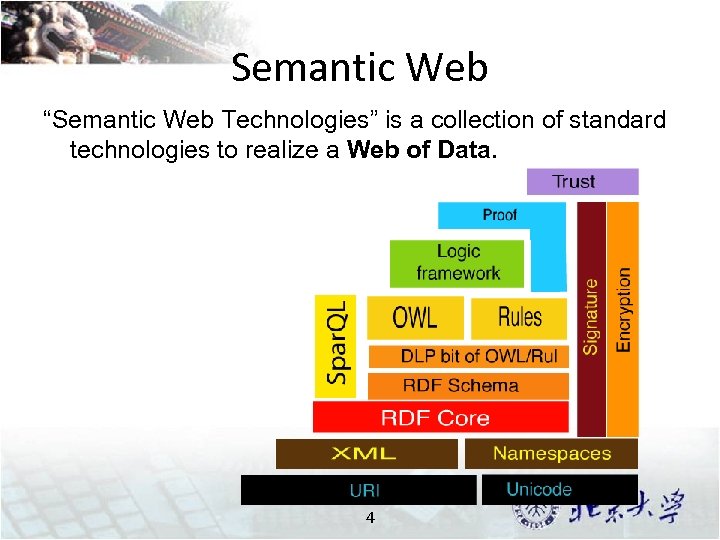
Semantic Web “Semantic Web Technologies” is a collection of standard technologies to realize a Web of Data. 4
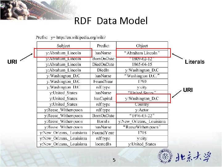
RDF Data Model URI Literals URI 5
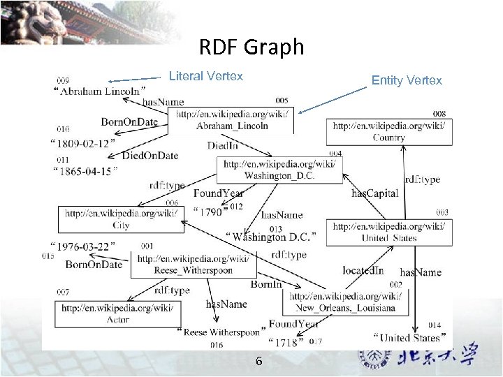
RDF Graph Literal Vertex Entity Vertex 6
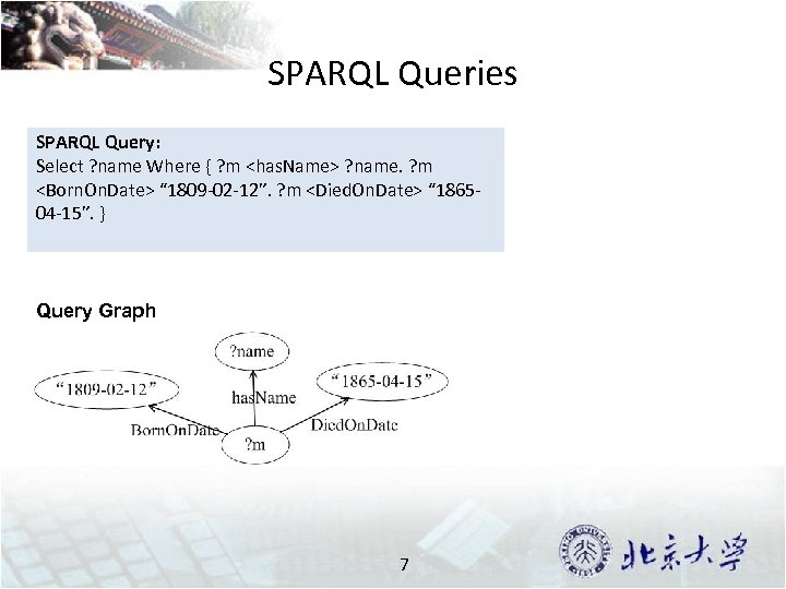
SPARQL Queries SPARQL Query: Select ? name Where { ? m <has. Name> ? name. ? m <Born. On. Date> “ 1809 -02 -12”. ? m <Died. On. Date> “ 186504 -15”. } Query Graph 7
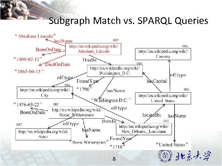
Subgraph Match vs. SPARQL Queries 8
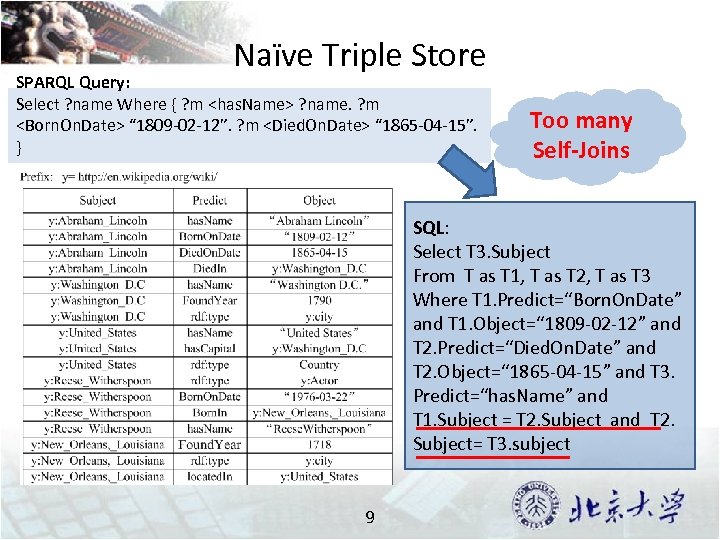
Naïve Triple Store SPARQL Query: Select ? name Where { ? m <has. Name> ? name. ? m <Born. On. Date> “ 1809 -02 -12”. ? m <Died. On. Date> “ 1865 -04 -15”. } Too many Self-Joins SQL: Select T 3. Subject From T as T 1, T as T 2, T as T 3 Where T 1. Predict=“Born. On. Date” and T 1. Object=“ 1809 -02 -12” and T 2. Predict=“Died. On. Date” and T 2. Object=“ 1865 -04 -15” and T 3. Predict=“has. Name” and T 1. Subject = T 2. Subject and T 2. Subject= T 3. subject 9
Existing Solutions Three categories of solutions are proposed to speed up query processing: 1. Property Table; Jena [K. Wilkinson et al. SWDB 03], … 2. Vertically Partitioned Solution; SW-store [D. J. Abadi et al. VLDB 07], … 3. Exhaustive-Indexing RDF-3 x [T. Neumann et al. VLDB 08], Hexastore [C. Weiss et al. VLDB 08 ], … 10
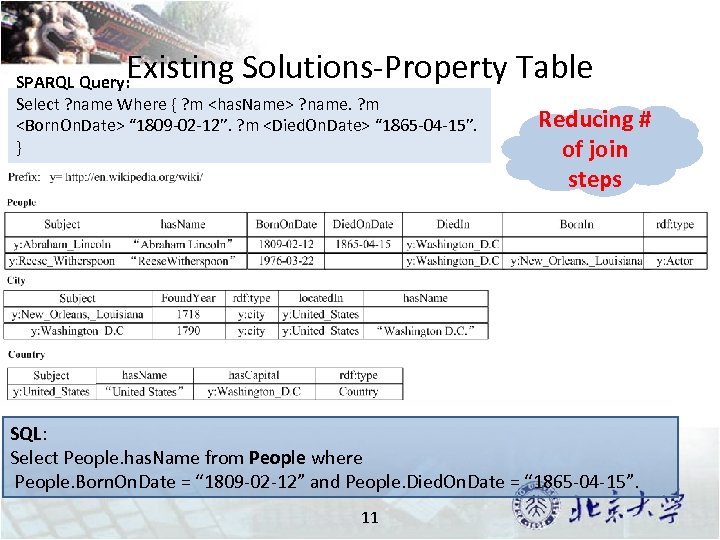
Existing Solutions-Property Table SPARQL Query: Select ? name Where { ? m <has. Name> ? name. ? m <Born. On. Date> “ 1809 -02 -12”. ? m <Died. On. Date> “ 1865 -04 -15”. } Reducing # of join steps SQL: Select People. has. Name from People where People. Born. On. Date = “ 1809 -02 -12” and People. Died. On. Date = “ 1865 -04 -15”. 11
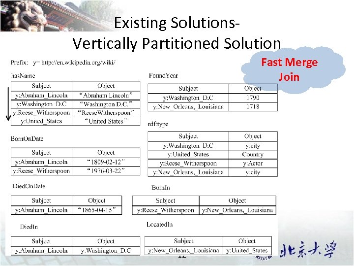
Existing Solutions. Vertically Partitioned Solution Fast Merge Join 12
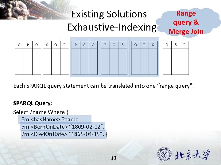
Existing Solutions. Exhaustive-Indexing Range query & Merge Join Each SPARQL query statement can be translated into one “range query”. SPARQL Query: Select ? name Where { ? m <has. Name> ? name. ? m <Born. On. Date> “ 1809 -02 -12”. ? m <Died. On. Date> “ 1865 -04 -15”. } 13
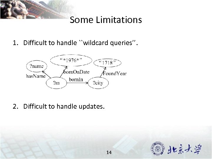
Some Limitations 1. Difficult to handle ``wildcard queries’’. 2. Difficult to handle updates. 14
Outline • Background & Related Work • Overview of g. Store • Encoding Technique • VS*-tree & Query Algorithm • Experiments • Conclusions 15
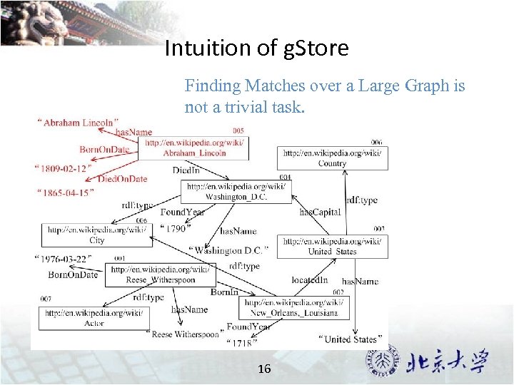
Intuition of g. Store Finding Matches over a Large Graph is not a trivial task. 16
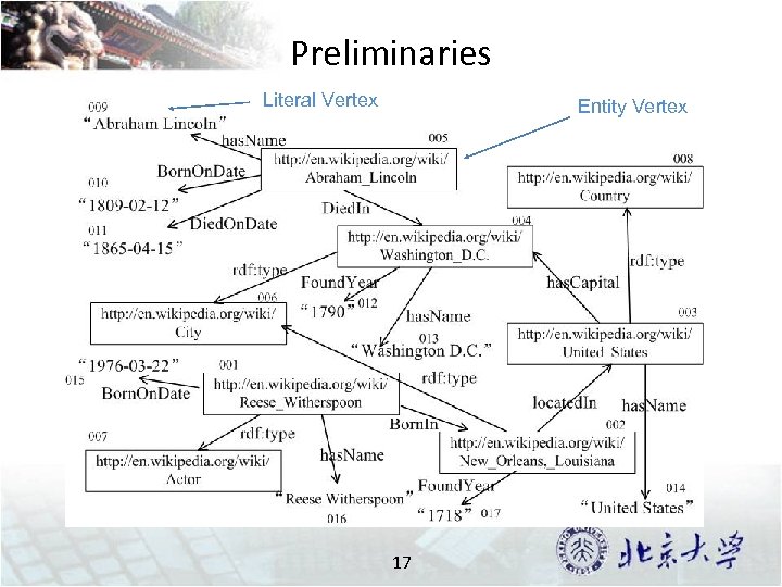
Preliminaries Literal Vertex Entity Vertex 17
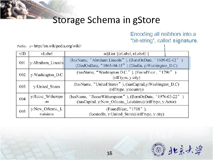
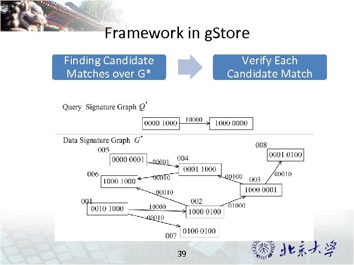
Storage Schema in g. Store Encoding all neibhors into a “bit-string”, called signature. 18
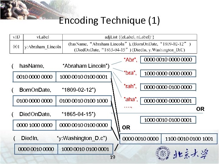
Encoding Technique (1) ( has. Name, 0010 0000 ( Born. On. Date, 0100 0000 ( Died. On. Date, 0000 1000 0000 ( Died. In, 0000 0010 0000 “Abr”, “bra”, “ 1809 -02 -12”) 0100 0010 0100 1000 0000 0100 0000 ”aha”, …. , 1000 0010 0100 0001 1000 0000 ”rah”, “Abraham Lincoln”) 0000 0010 0000 0001 “ 1865 -04 -15”) OR 1000 0010 0100 0001 0000 0010 0100 0000 OR “y: Washington_D. c”) 0000 0010 0000 1000 0010 0100 0001 19 1100 0010 0100 1001
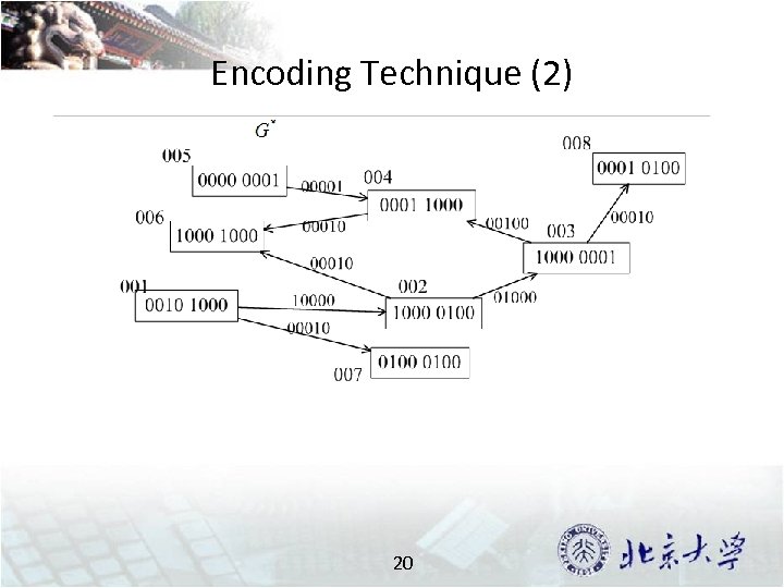
Encoding Technique (2) 20
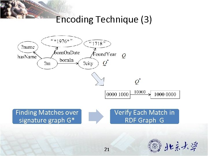
Encoding Technique (3) Finding Matches over signature graph G* Verify Each Match in RDF Graph G 21
Outline • Background & Related Work • Overview of g. Store • Encoding Technique • VS-tree & Query Algorithm • Experiments • Conclusions 22
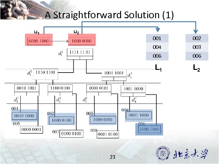
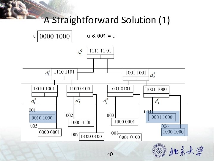
A Straightforward Solution (1) u 1 u 2 001 004 003 006 L 1 23 002 L 2
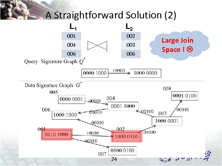
A Straightforward Solution (2) L 1 L 2 001 002 004 003 006 24 Large Join Space !
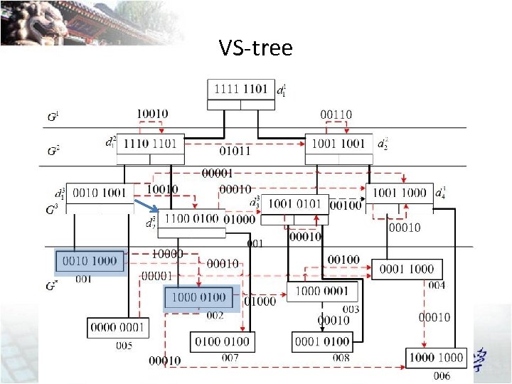
VS-tree
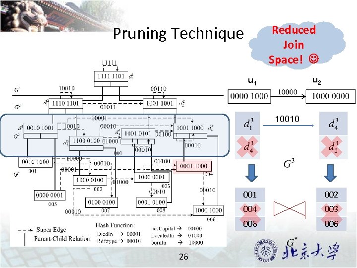
Reduced Join Space! Pruning Technique u 2 u 1 10010 001 004 003 006 26 002 006
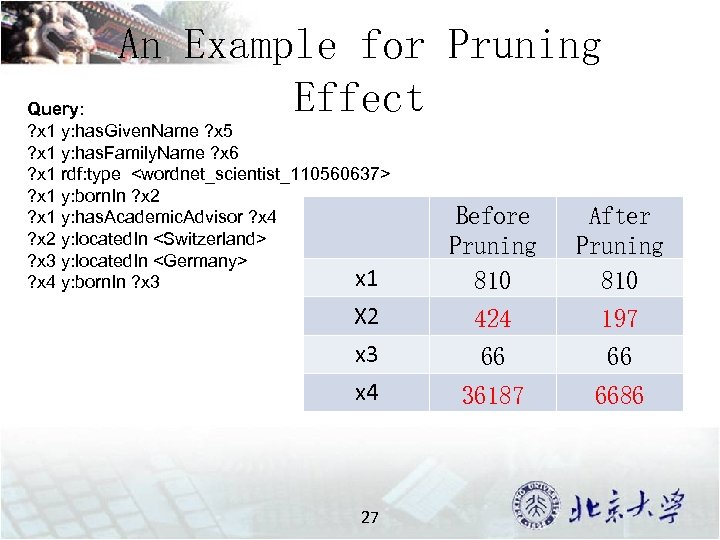
An Example for Pruning Effect Query: ? x 1 y: has. Given. Name ? x 5 ? x 1 y: has. Family. Name ? x 6 ? x 1 rdf: type <wordnet_scientist_110560637> ? x 1 y: born. In ? x 2 ? x 1 y: has. Academic. Advisor ? x 4 ? x 2 y: located. In <Switzerland> ? x 3 y: located. In <Germany> x 1 ? x 4 y: born. In ? x 3 Before Pruning 810 After Pruning 810 X 2 424 197 x 3 66 66 x 4 36187 6686 27
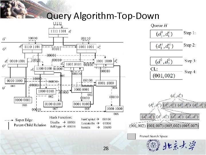
Query Algorithm-Top-Down 28
Outline • Background & Related Work • Overview of g. Store • Encoding Technique • VS*-tree & Query Algorithm • Experiments • Conclusions 29
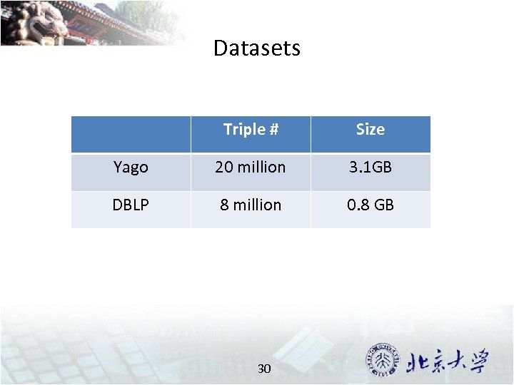
Datasets Triple # Size Yago 20 million 3. 1 GB DBLP 8 million 0. 8 GB 30
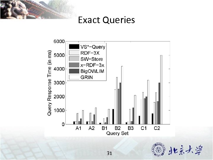
Exact Queries 31
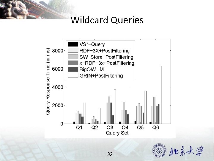
Wildcard Queries 32
Outline • Background & Related Work • Overview of g. Store • Encoding Technique • VS*-tree & Query Algorithm • Experiments • Conclusions 33
Conclusions • Vertex Encoding Technique; • An Efficient index Structure: VS-tree; • A Novel Filtering Technique. 34

Q/A Thank You! zoulei@pku. edu. cn 35
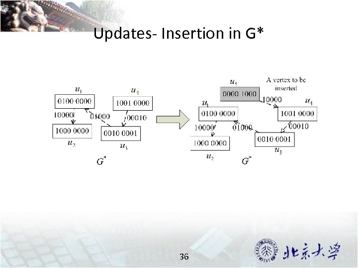
Updates- Insertion in G* 36
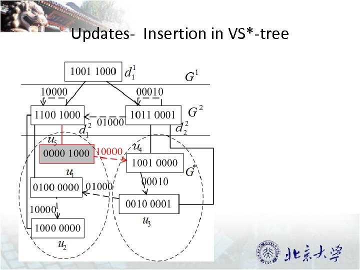
Updates- Insertion in VS*-tree 37
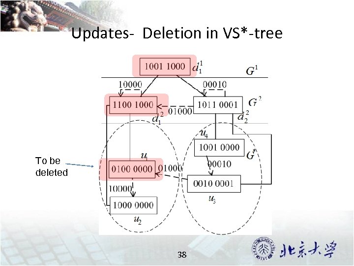
Updates- Deletion in VS*-tree To be deleted 38
Framework in g. Store Finding Candidate Matches over G* Verify Each Candidate Match 39
A Straightforward Solution (1) u u & 001 = u 40
0007804a8c3edd045bd7ebed8417f385.ppt