G-commerce Computational economies for resource allocation in computational

G-commerce Computational economies for resource allocation in computational Grid settings Fundamentals n n n Resources are not free For convincing resource owners to federate their resources for the Grid The relative worth of a resource is determined by its supply and demand for it. 2 economic models n n Commodities markets – natural since applications treat resources as commodities Auctions – easy to implement Evaluation criteria n n Price stability – i. e. fluctuations of price – price stability for scheduling stability Equilibrium – degree to which prices are fair – trustworthiness Application efficiency Resource efficiency

Commodity Markets and Auctions Commodity Markets n n n A third-party (market) sets a price for resources and asks producers and consumers willing to agree to that price The participants engage in transactions Based on unsatisfied demands and supplies, new prices are set Consumers don’t ask for specific commodity but chooses one out of many equivalents An attempt is made to satisfy all bidders and sellers at a given price Auctions n n n A third-party (auctioneer) collects resources and bids Highest bidder gets a resource per auction round Prices are set based on bids Process repeated for other resources Consumers ask for specific commodities One bidder and one seller satisfied at a given price

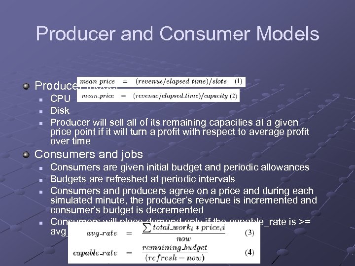Producer and Consumer Models Producer model n n n CPU Disk Producer will sell all of its remaining capacities at a given price point if it will turn a profit with respect to average profit over time Consumers and jobs n n Consumers are given initial budget and periodic allowances Budgets are refreshed at periodic intervals Consumers and producers agree on a price and during each simulated minute, the producer’s revenue is incremented and consumer’s budget is decremented Consumers will place demand only if the capable_rate is >= avg_rate

Producer and Consumer Models Summary n n n Producers consider long term profit and past performance when deciding to sell Consumers are given periodic budget replenishments and spend opportunistically Consumers introduce work load in bulk at the beginning of each simulated day, and randomly throughout the day

Commodities market and dynamic pricing Pricing methodology for market economy Pricing methodology should produce a system of price adjustments which bring about market equilibrium Market economy is a system involving producers, consumers, several commodities, supply and demand functions for each commodity determined by the set of market prices for various commodities A unique equilibrium price is guaranteed to exist in this framework

Commodities Commodity prices represented by price vector, p. zj - Excess demand for the jth commodity, i. e. demand minus supply Each zj is a function of all prices pi Smale’s theorem: an equilibrium point with p* such that excess demand vector z(p*) = 0 exists

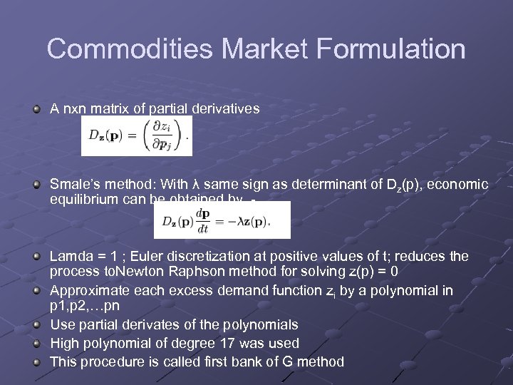Commodities Market Formulation A nxn matrix of partial derivatives Smale’s method: With λ same sign as determinant of Dz(p), economic equilibrium can be obtained by - Lamda = 1 ; Euler discretization at positive values of t; reduces the process to. Newton Raphson method for solving z(p) = 0 Approximate each excess demand function zi by a polynomial in p 1, p 2, …pn Use partial derivates of the polynomials High polynomial of degree 17 was used This procedure is called first bank of G method

Auctions When an application desires multiple commodities, it places multiple bids on multiple auctions and obtains some of the resources It expends currency on the obtained resources while it waits for other resources Auctions are highly unreliable in terms of pricing and ability to obtain resource – leads to poor scheduling decisions

Simulations of auctions At each time step, CPU and disk producers submit their unused slots, minimum selling price (average profit / slot) to auctioneers Consumers define bid prices based on demand functions and bid on each commodity needed by their jobs Highest bidding customer gets commodity Price of the commodity – average of commodity’s minimum selling price and consumer’s bid price

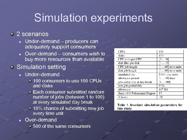Simulation experiments 2 scenarios n n Under-demand – producers can adequately support consumers Over-demand – consumers wish to buy more resources than available Simulation setting n Under-demand 100 consumers to use 100 CPUs and disks Each consumer submitted random number of jobs (between 1 to 100) at every simulated day break 10% chance of submitting new job every time unit n Over-demand 500 of the same consumers

Market equilibrium – commodity markets: Illustration of equilibrium by Smale’s method

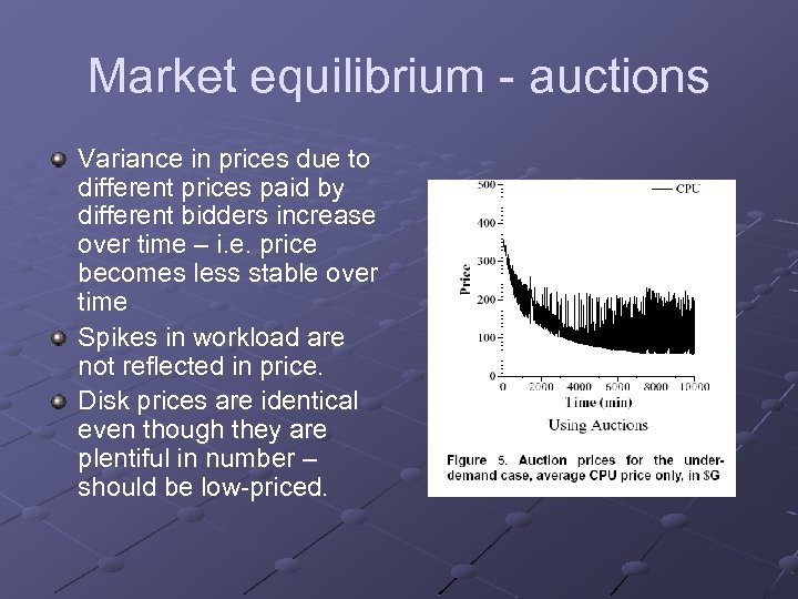Market equilibrium - auctions Variance in prices due to different prices paid by different bidders increase over time – i. e. price becomes less stable over time Spikes in workload are not reflected in price. Disk prices are identical even though they are plentiful in number – should be low-priced.

Market equilibrium - Summary Smale’s method is appropriate for modeling hypothetical Grid market First bank of G reasonable and implementable approximation Auctioneering attractive from implementation standpoint But does not produce stable pricing or market equilibrium Grid resource allocation decisions based on auctioneering lack fairness Commodities market formulation perform better from the standpoint of Grid as a whole Over-demand case performed similar to under-demand

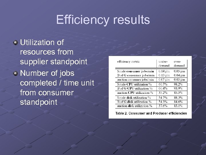Efficiency results Utilization of resources from supplier standpoint Number of jobs completed / time unit from consumer standpoint

Other Pricing Models Posted Price Model n Special offers to motivate users to utilize unused slots Bargaining Model Tender/contract-net model Bid-based proportional resource sharing model n Used in cooperative resource sharing environments Share-holders model n When users are both service providers and consumers Monopoly

An Incentive-based Grid Scheduling Resource Consumers n Job length, job deadline Resource Providers n Capability, unit price and job queue Scheduling objective n n Provide Qo. S to consumers. Highly successful (without missing deadline) execution rate of job Reasonable profit for providers. Fair allocation of benefits, i. e. the profit of every provider is proportional to its investment or cost

Overall Design Peer-2 -peer grid Step 1 – a consumer submits job announcement, broadcast to all providers Step 2 - Provider estimates whether it is able to meet deadline. Yes- provider sends a bid containing the charge for the job Step 3 - Consumer processes all the bids and chooses the provider with the least charge. Sends job Step 4 - Provider queues it, executes and sends results

Job Competing Algorithm for Step 2 How a provider bids. Job competing algorithm After a provider has sent its bid to previous job (unconfirmed job), when a job announcement comes for a new job, should it consider the previous job for deciding on whether to bid for the new job? Parameter α, conservation degree α = 0, aggressive. Don’t consider unconfirmed jobs when estimating whether it will meet a new job deadline α = 1, conservative. Consider unconfirmed jobs when estimating whether it will meet a new job deadline

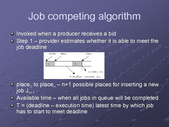Job competing algorithm Invoked when a producer receives a bid Step 1 – provider estimates whether it is able to meet the job deadline place 0 to placen – n+1 possible places for inserting a new job Jn+1 Available time – when all jobs in queue will be completed T = (deadline – execution time) latest time by which job has to start to meet deadline

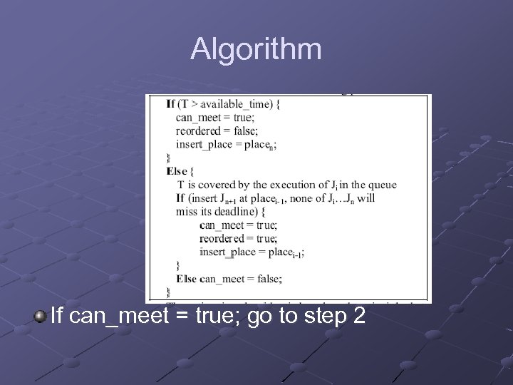Algorithm If can_meet = true; go to step 2

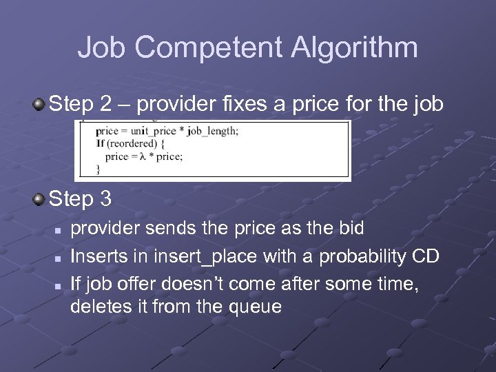Job Competent Algorithm Step 2 – provider fixes a price for the job Step 3 n n n provider sends the price as the bid Inserts in insert_place with a probability CD If job offer doesn’t come after some time, deletes it from the queue

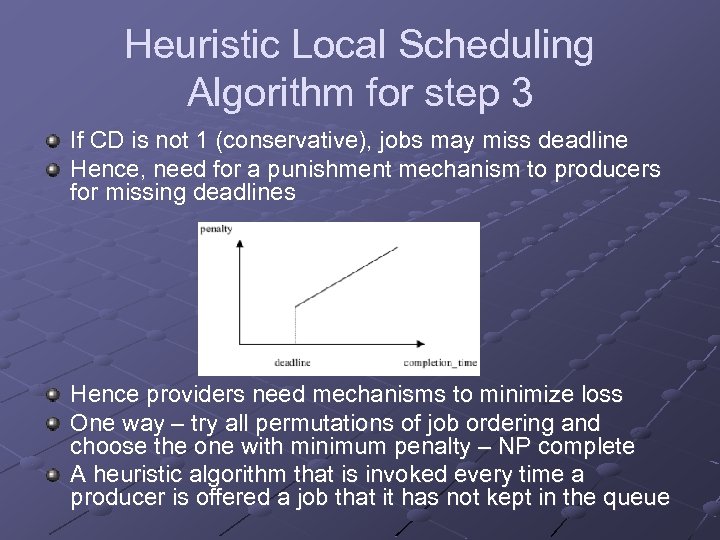Heuristic Local Scheduling Algorithm for step 3 If CD is not 1 (conservative), jobs may miss deadline Hence, need for a punishment mechanism to producers for missing deadlines Hence providers need mechanisms to minimize loss One way – try all permutations of job ordering and choose the one with minimum penalty – NP complete A heuristic algorithm that is invoked every time a producer is offered a job that it has not kept in the queue

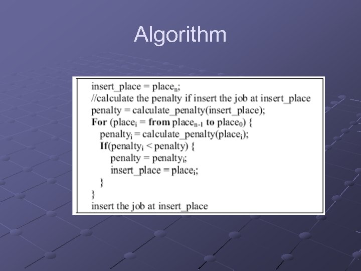Algorithm

Price Adjustments Initially, a market price for a commodity is fixed When a provider enters the grid, gets this market price and uses it as initial unit price Every time a provider is offered a job or deletes an unconfirmed job, invokes the price adjustment algorithm

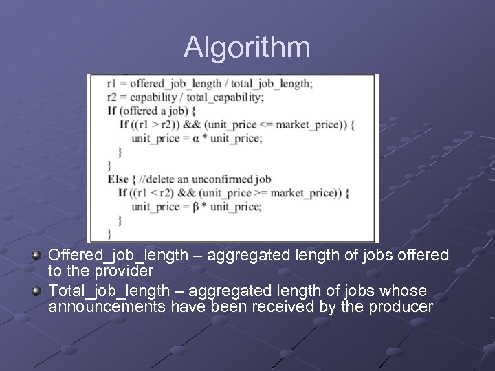Algorithm Offered_job_length – aggregated length of jobs offered to the provider Total_job_length – aggregated length of jobs whose announcements have been received by the producer

Simulation Setup 20 consumers, 80 producers Fixed values for n n n Average lengths of jobs Average of capabilities of providers λ, α, β Market price Different system loads CD – 0, 0. 5, 1

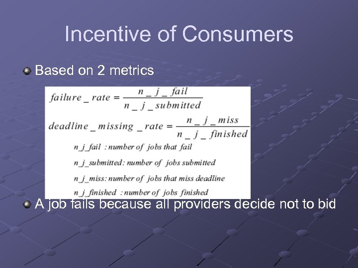Incentive of Consumers Based on 2 metrics A job fails because all providers decide not to bid

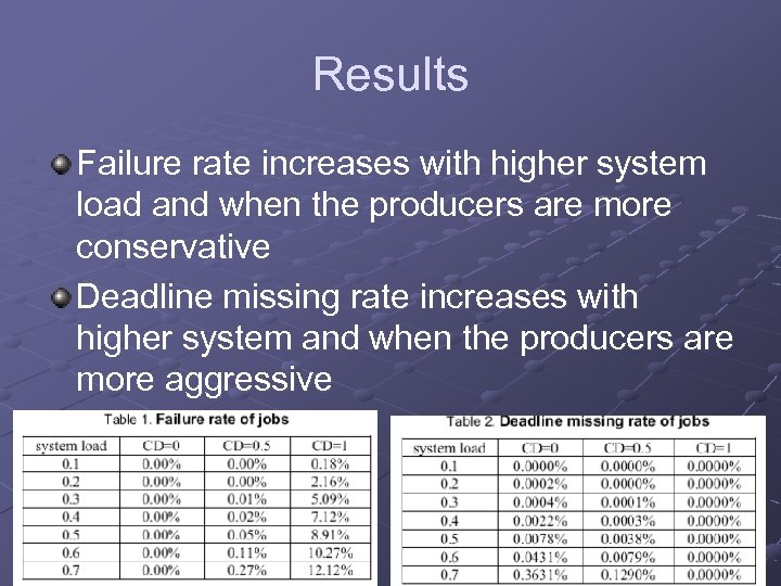Results Failure rate increases with higher system load and when the producers are more conservative Deadline missing rate increases with higher system and when the producers are more aggressive

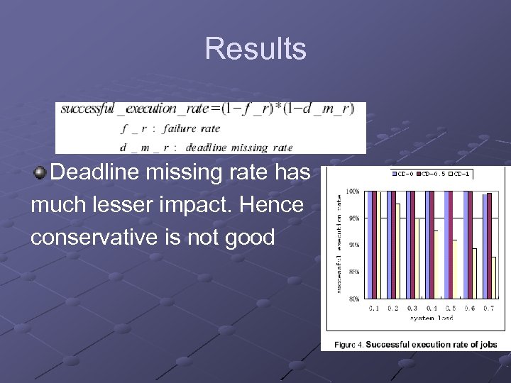Results Deadline missing rate has much lesser impact. Hence conservative is not good

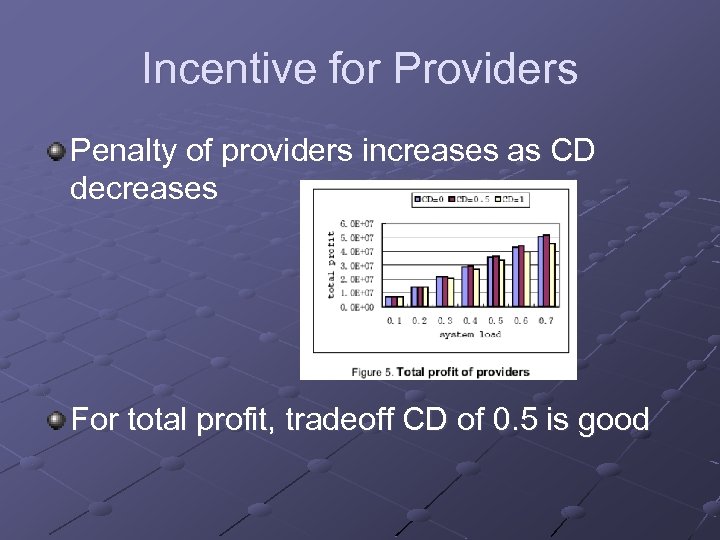Incentive for Providers Penalty of providers increases as CD decreases For total profit, tradeoff CD of 0. 5 is good

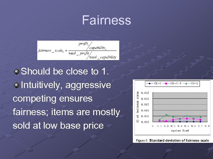Fairness Should be close to 1. Intuitively, aggressive competing ensures fairness; items are mostly sold at low base price

Game-Theory Based Pricing Strategy Pricing strategy implemented between job allocator and nodes using game theoretic framework The 2 players are job allocator and nodes They play incomplete information, alternatingoffers, noncooperative, bargaining game to decide on n n Price per unit resource Percentage of bandwidth that can be used on the link between job allocator and nodes If there are n nodes, a JA plays a game with each of the n nodes to form vectors of price and percentage bandwidth

Incomplete Information Two players have no idea of each other’s reserved valuations JA n n Maximum offered price Minimum bandwidth percentage Node n n Minimum expected price Maximum bandwidth percentage Both can make surplus or profit and try to reach a mutually beneficial arrangement

Rules for JA Rule 1 – at each step of the game, both players choose the alternative earning them highest expected price Expected utility = [(reserved valuation of JA – offered price) + (offered percentage of bandwidth – minimum percentage)] x probability(offered price, percentage of bandwidth offered) Probability – that the tuple will be accepted by the opponent

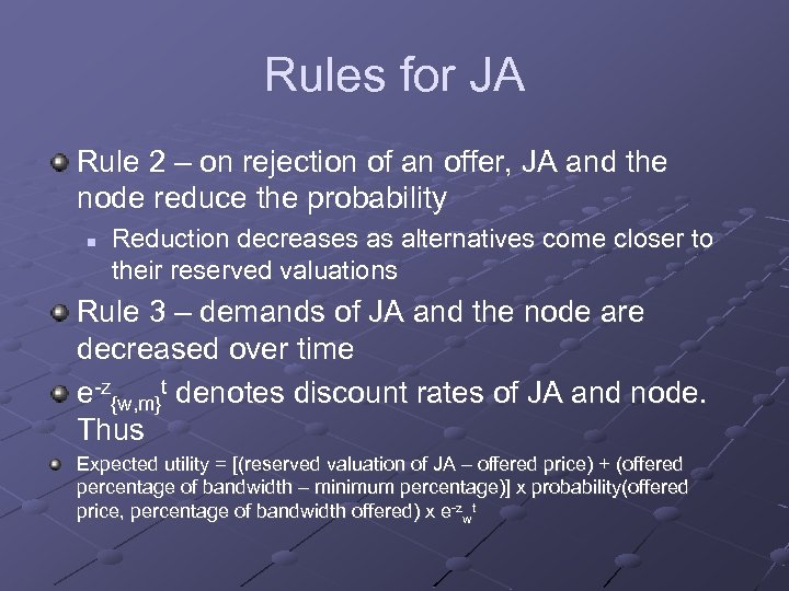Rules for JA Rule 2 – on rejection of an offer, JA and the node reduce the probability n Reduction decreases as alternatives come closer to their reserved valuations Rule 3 – demands of JA and the node are decreased over time e-z{w, m}t denotes discount rates of JA and node. Thus Expected utility = [(reserved valuation of JA – offered price) + (offered percentage of bandwidth – minimum percentage)] x probability(offered price, percentage of bandwidth offered) x e-zwt

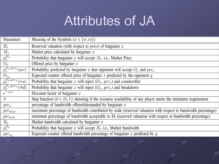Attributes of JA

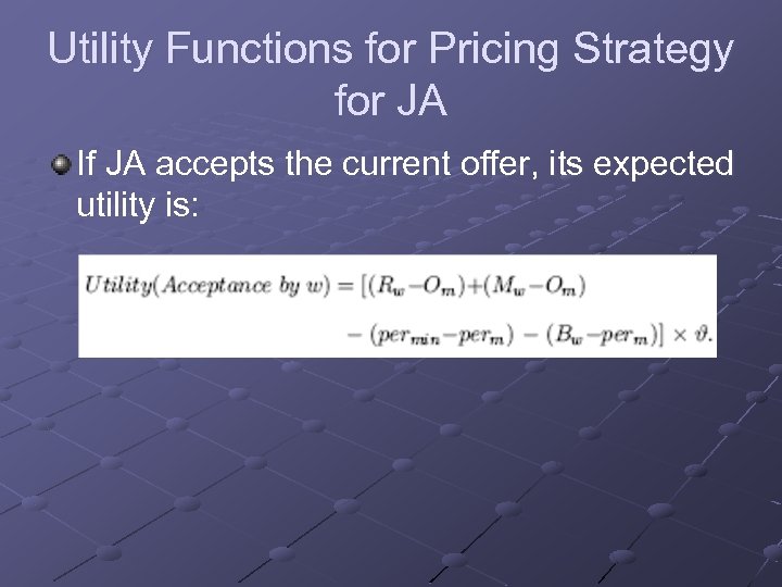Utility Functions for Pricing Strategy for JA If JA accepts the current offer, its expected utility is:

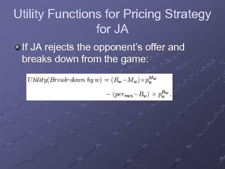Utility Functions for Pricing Strategy for JA If JA rejects the opponent’s offer and breaks down from the game:

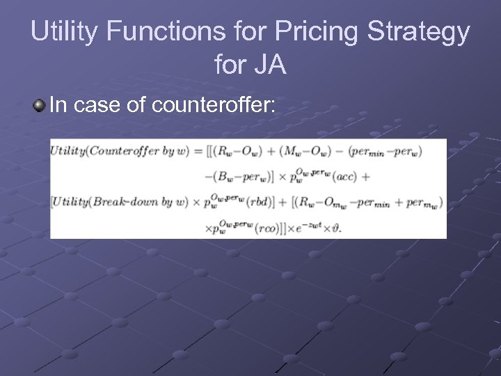Utility Functions for Pricing Strategy for JA In case of counteroffer:

References / Sources / Credits Wolski, R. , Plank, J. , Brevik, J, and Bryan, T. , GCommerce: Market Formulations Controlling Resource Allocation on the Computational Grid (PDF), IPDPS 01, March, 2001. Buyya et. al. Economic Models for Resource Management and Scheduling in Grid Computing. Concurrency and Computation. Practice and Experience. 2002. 14: 1507 -1542. Grid. IS: An Incentive Based Grid Scheduling. Xiao et. al. IPDPS 2005 A Game Theory-Based Pricing Strategy to Support Single/Multiclass Job Allocation Schemes for Bandwidth. Constrained Distributed Computing Systems. Ghosh et. al. TPDS 2007.

JUNK!

Differences In commodity markets, an attempt is made to satisfy all bidders and sellers at a given price In auctions, one bidder and seller is satisfied at a given price