FX Derivatives 3 Hedging Exposure FX Risk

FX Derivatives 3. Hedging Exposure

FX Risk Management Exposure At the firm level, currency risk is called exposure. Three areas (1) Transaction exposure: Risk of transactions denominated in FX with a payment date or maturity. (2) Economic exposure: Degree to which a firm's expected cash flows are affected by unexpected changes in St. (3) Translation exposure: Accounting based changes in a firm's consolidated statements that result from a change in St. Translation rules are complicated: Not all items are translated using the same St. These rules create accounting gains/losses due to changes in St. We will say a firm is “exposed” or has exposure if it faces currency risk.

Q: How can FX changes affect the firm? Transaction Exposure Short term CFs: Existing contract obligations. Economic Exposure Future CFs: Erosion of competitive position. Translation Exposure Revaluation of balance sheet (Book Value vs Market Value).

Example: Exposure. A. Transaction exposure. Swiss Cruises, a Swiss firm, sells cruise packages priced in USD to a broker. Payment in 30 days. B. Economic exposure. Swiss Cruises has 50% of its revenue denominated in USD and only 20% of its cost denominated in USD. A depreciation of the USD will affect future CHF cash flows. C. Translation exposure. Swiss Cruises obtains a USD loan from a U. S. bank. This liability has to be translated into CHF following Swiss accounting rules. ¶

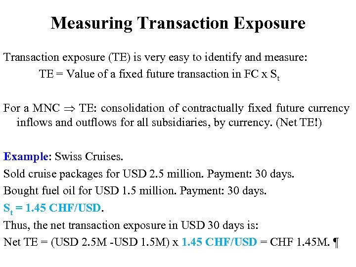Measuring Transaction Exposure Transaction exposure (TE) is very easy to identify and measure: TE = Value of a fixed future transaction in FC x St For a MNC TE: consolidation of contractually fixed future currency inflows and outflows for all subsidiaries, by currency. (Net TE!) Example: Swiss Cruises. Sold cruise packages for USD 2. 5 million. Payment: 30 days. Bought fuel oil for USD 1. 5 million. Payment: 30 days. St = 1. 45 CHF/USD. Thus, the net transaction exposure in USD 30 days is: Net TE = (USD 2. 5 M USD 1. 5 M) x 1. 45 CHF/USD = CHF 1. 45 M. ¶

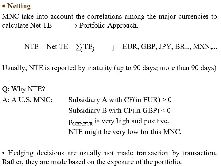Netting MNC take into account the correlations among the major currencies to calculate Net TE Portfolio Approach. NTE = Net TE = ∑j TEj j = EUR, GBP, JPY, BRL, MXN, . . . Usually, NTE is reported by maturity (up to 90 days; more than 90 days) Q: Why NTE? A: A U. S. MNC: Subsidiary A with CF(in EUR) > 0 Subsidiary B with CF(in GBP) < 0 GBP, EUR is very high and positive. NTE might be very low for this MNC. • Hedging decisions are usually not made transaction by transaction. Rather, they are made based on the exposure of the portfolio.

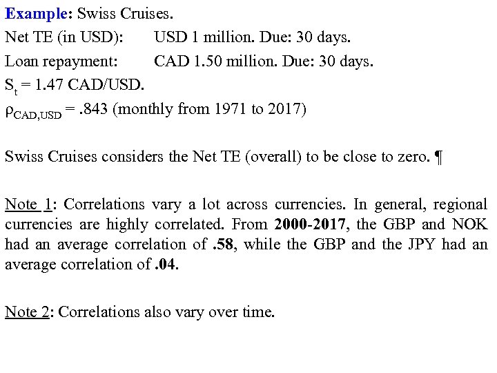Example: Swiss Cruises. Net TE (in USD): USD 1 million. Due: 30 days. Loan repayment: CAD 1. 50 million. Due: 30 days. St = 1. 47 CAD/USD. CAD, USD =. 843 (monthly from 1971 to 2017) Swiss Cruises considers the Net TE (overall) to be close to zero. ¶ Note 1: Correlations vary a lot across currencies. In general, regional currencies are highly correlated. From 2000 -2017, the GBP and NOK had an average correlation of . 58, while the GBP and the JPY had an average correlation of. 04. Note 2: Correlations also vary over time.

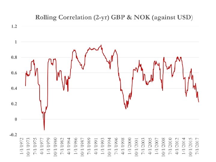
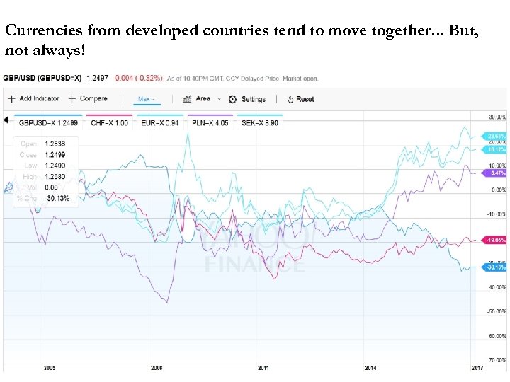Currencies from developed countries tend to move together. . . But, not always!

• Q: How does TE affect a firm in the future? MNCs are interested in how TE will change in the future (say, in T days). After all, it is in the future that the transaction will be settled. MNCs do not know the future St+T, they need to forecast St+T. Et[St+T] has an associated standard error, which produces a range for (or an interval around ) St+T and, thus, TE. From a risk management perspective, it is important to know how much will be received from a FC inflow or how much will be needed to cover a FC outflow.

Range Estimates of TE • St is very difficult to forecast. Thus, a range estimate of the Net TE will provide a more useful number for risk managers. The smaller the range, the lower the sensitivity of the Net TE. • Three popular methods for estimating a range for Net TE: (1) Ad hoc rule (say, ± 10%) (2) Sensitivity Analysis (or simulating exchange rates) (3) Assuming a statistical distribution for exchange rates.

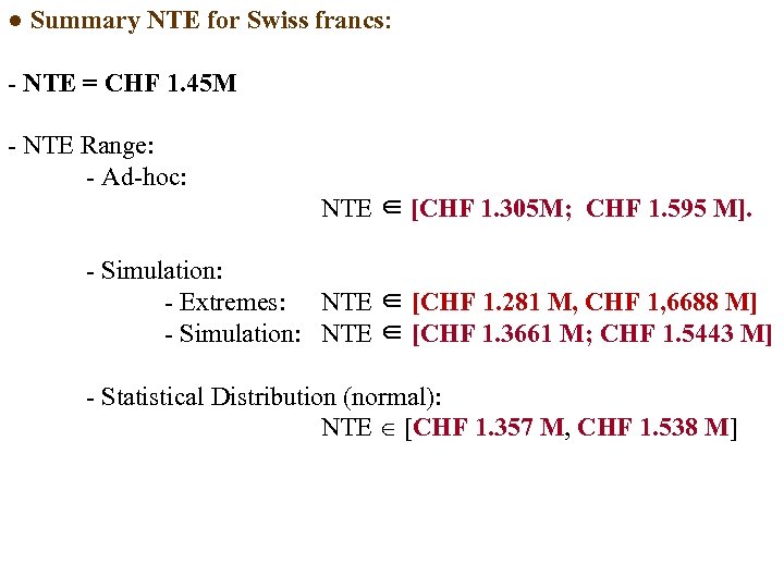
Ad-hoc Rule Instead of using a specific confidence interval (C. I. ), which requires (complicated calculations and/or unrealistic assumptions) many firms use an ad hoc rule to get a range: ±X% (for example, a 10% rule) It’s a simple and easy to understand: Get TE and add/subtract ±X%. Example: 10% Rule. SC has a Net TE= CHF 1. 45 M due in 30 days ⇒ if St changes by ± 10%, Net TE changes by ± CHF 145, 000. ¶ Note: This example gives a range for NTE: NTE ∈ [CHF 1. 305 M; CHF 1. 595 M] ⇒ wider range: riskier exposure. Risk Management Interpretation: If SC is counting on the USD 1 M to pay CHF expenses, these expenses should not exceed CHF 1. 305 M. ¶

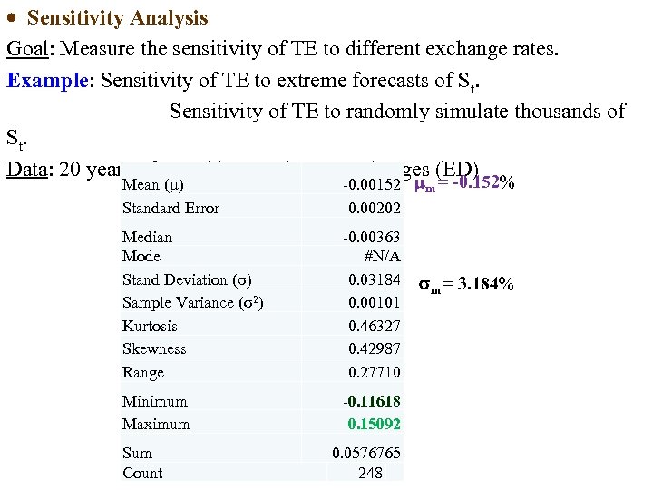Sensitivity Analysis Goal: Measure the sensitivity of TE to different exchange rates. Example: Sensitivity of TE to extreme forecasts of St. Sensitivity of TE to randomly simulate thousands of St. Data: 20 years of monthly CHF/USD % changes (ED) Mean ( ) Standard Error 0. 00152 m = -0. 152% 0. 00202 Median Mode Stand Deviation (σ) Sample Variance (σ2) Kurtosis Skewness Range 0. 00363 #N/A 0. 03184 0. 00101 0. 46327 0. 42987 0. 27710 Minimum Maximum 0. 11618 0. 15092 Sum Count 0. 0576765 248 m = 3. 184%

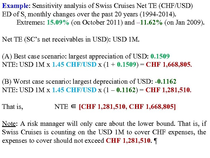Example: Sensitivity analysis of Swiss Cruises Net TE (CHF/USD) ED of St monthly changes over the past 20 years (1994 2014). Extremes: 15. 09% (on October 2011) and – 11. 62% (on Jan 2009). Net TE (SC’s net receivables in USD): USD 1 M. (A) Best case scenario: largest appreciation of USD: 0. 1509 NTE: USD 1 M x 1. 45 CHF/USD x (1 + 0. 1509) = CHF 1, 668, 805. (B) Worst case scenario: largest depreciation of USD: -0. 1162 NTE: USD 1 M x 1. 45 CHF/USD x (1 – 0. 1162) = CHF 1, 281, 510. That is, NTE ∈ [CHF 1, 281, 510, CHF 1, 668, 805] Note: A risk manager will only care about the lower bound. That is, if Swiss Cruises is counting on the USD 1 M to cover CHF expenses, the expenses to cover should not exceed CHF 1, 281, 510. ¶

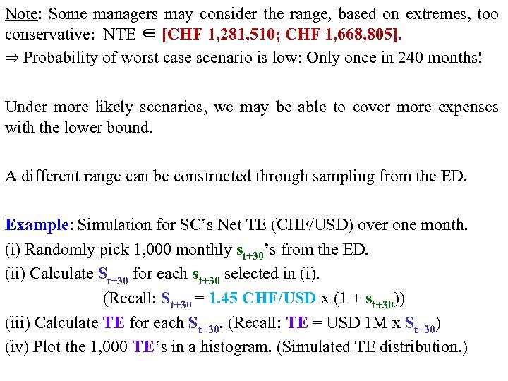Note: Some managers may consider the range, based on extremes, too conservative: NTE ∈ [CHF 1, 281, 510; CHF 1, 668, 805]. ⇒ Probability of worst case scenario is low: Only once in 240 months! Under more likely scenarios, we may be able to cover more expenses with the lower bound. A different range can be constructed through sampling from the ED. Example: Simulation for SC’s Net TE (CHF/USD) over one month. (i) Randomly pick 1, 000 monthly st+30’s from the ED. (ii) Calculate St+30 for each st+30 selected in (i). (Recall: St+30 = 1. 45 CHF/USD x (1 + st+30)) (iii) Calculate TE for each St+30. (Recall: TE = USD 1 M x St+30) (iv) Plot the 1, 000 TE’s in a histogram. (Simulated TE distribution. )

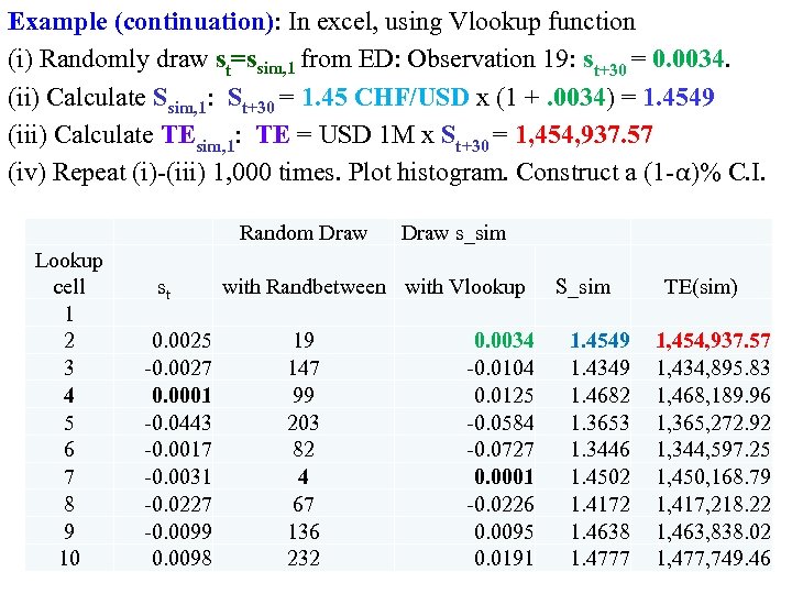Example (continuation): In excel, using Vlookup function (i) Randomly draw st=ssim, 1 from ED: Observation 19: st+30 = 0. 0034. (ii) Calculate Ssim, 1: St+30 = 1. 45 CHF/USD x (1 +. 0034) = 1. 4549 (iii) Calculate TEsim, 1: TE = USD 1 M x St+30 = 1, 454, 937. 57 (iv) Repeat (i) (iii) 1, 000 times. Plot histogram. Construct a (1 α)% C. I. Random Draw Lookup cell 1 2 3 4 5 6 7 8 9 10 st 0. 0025 0. 0027 0. 0001 0. 0443 0. 0017 0. 0031 0. 0227 0. 0099 0. 0098 Draw s_sim with Randbetween with Vlookup 19 147 99 203 82 4 67 136 232 0. 0034 0. 0104 0. 0125 0. 0584 0. 0727 0. 0001 0. 0226 0. 0095 0. 0191 S_sim 1. 4549 1. 4349 1. 4682 1. 3653 1. 3446 1. 4502 1. 4172 1. 4638 1. 4777 TE(sim) 1, 454, 937. 57 1, 434, 895. 83 1, 468, 189. 96 1, 365, 272. 92 1, 344, 597. 25 1, 450, 168. 79 1, 417, 218. 22 1, 463, 838. 02 1, 477, 749. 46

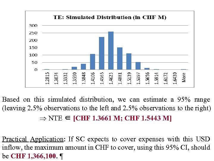Based on this simulated distribution, we can estimate a 95% range (leaving 2. 5% observations to the left and 2. 5% observations to the right) NTE ∈ [CHF 1. 3661 M; CHF 1. 5443 M] Practical Application: If SC expects to cover expenses with this USD inflow, the maximum amount in CHF to cover, using this 95% CI, should be CHF 1, 366, 100. ¶

Aside: How many draws in the simulations? Usually, we draw until the histograms –i. e. , CIs– do not change a lot. Example: 1, 000 and 10, 000 draws For the SC example, we drew 1, 000 scenarios to get a 95% C. I. : NTE ∈ [CHF 1. 3661 M; CHF 1. 5443 M] Now, we draw 10, 000 scenarios and determined the following 95% C. I. : NTE ∈ [CHF 1. 3670 M; CHF 1. 5446 M]

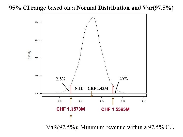
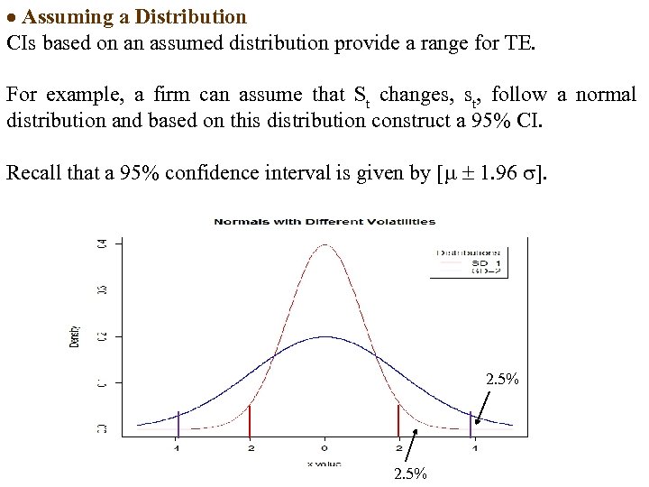Assuming a Distribution CIs based on an assumed distribution provide a range for TE. For example, a firm can assume that St changes, st, follow a normal distribution and based on this distribution construct a 95% CI. Recall that a 95% confidence interval is given by [ 1. 96 ]. 2. 5%

Example: CI range based on a Normal distribution. Assume Swiss Cruises believes that CHF/USD monthly changes follow a normal distribution. Swiss Cruises estimates the mean and the variance. = Monthly mean = -0. 00152 ≈ 0. 15% 2 = Monthly variance = 0. 001014 ( = 0. 03184, or 3. 18%) st ~ N( 0. 00152, 0. 001014). st = CHF/USD monthly changes. Swiss Cruises constructs a 95% CI for CHF/USD monthly changes. Recall that a 95% confidence interval is given by: [-0. 00152 1. 96*0. 03184] = [ 0. 06393; 0. 06089]. Based on this range for st, we derive bounds for the net TE: (A) Upper bound NTE: USD 1 M x 1. 45 CHF/USD x (1 + 0. 06089) = CHF 1, 538, 291. (B) Lower bound

95% CI range based on a Normal Distribution and Var(97. 5%) 2. 5% NTE = CHF 1. 45 M CHF 1. 3573 M CHF 1. 5383 M Va. R(97. 5%): Minimum revenue within a 97. 5% C. I.

NTE [CHF 1. 357 M, CHF 1. 538 M] • The lower bound, for a receivable, represents the worst case scenario within the confidence interval. There is a Value-at-Risk (Va. R) interpretation: Va. R: Maximum expected loss in a given time interval within a (one sided) CI. In our case, we can express the “expected loss” relative to today’s value: Va. R mean: Va. R – Net TE Example (continuation): Va. R(97. 5%) = CHF 1, 357, 302, the minimum revenue to be received by SC in the next 30 days, within a 97. 5% CI. Then, Va. R mean (97. 5%) = CHF 1. 3573 M – CHF 1. 45 M = CHF -0. 0927 M

• Summary NTE [CHF 1. 357 M, CHF 1. 538 M] Va. R(97. 5%) = CHF 1, 357, 302 If SC expects to cover expenses with this USD inflow, the maximum amount in CHF to cover, within a 97. 5% CI, should be CHF 1, 357, 302. Va. R mean (97. 5%) = CHF 0. 09527 M Relative to today’s valuation (or expected valuation, according to RWM), the maximum expected loss with a 97. 5% “chance” is CHF 0. 0927 M. ¶

● Summary NTE for Swiss francs: NTE = CHF 1. 45 M NTE Range: Ad hoc: NTE ∈ [CHF 1. 305 M; CHF 1. 595 M]. Simulation: Extremes: NTE ∈ [CHF 1. 281 M, CHF 1, 6688 M] Simulation: NTE ∈ [CHF 1. 3661 M; CHF 1. 5443 M] Statistical Distribution (normal): NTE [CHF 1. 357 M, CHF 1. 538 M]

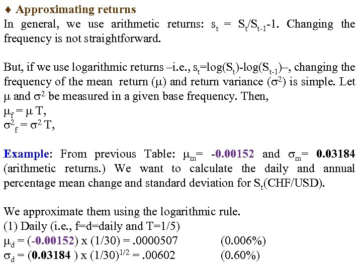Approximating returns In general, we use arithmetic returns: st = St/St 1 1. Changing the frequency is not straightforward. But, if we use logarithmic returns –i. e. , st=log(St) log(St 1)–, changing the frequency of the mean return ( ) and return variance ( 2) is simple. Let and 2 be measured in a given base frequency. Then, f = T, 2 f = 2 T, Example: From previous Table: m= 0. 00152 and m= 0. 03184 (arithmetic returns. ) We want to calculate the daily and annual percentage mean change and standard deviation for St(CHF/USD). We approximate them using the logarithmic rule. (1) Daily (i. e. , f=d=daily and T=1/5) d = (-0. 00152) x (1/30) =. 0000507 (0. 006%) d = (0. 03184 ) x (1/30)1/2 =. 00602 (0. 60%)

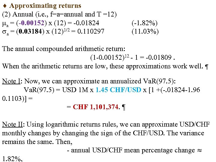Approximating returns (2) Annual (i. e. , f=a=annual and T =12) a = (-0. 00152) x (12) = 0. 01824 a = (0. 03184) x (12)1/2 = 0. 110297 ( 1. 82%) (11. 03%) The annual compounded arithmetic return: (1 0. 00152)12 1 = 0. 01809. When the arithmetic returns are low, these approximations work well. ¶ Note I: Now, we can approximate an annualized Va. R(97. 5): Va. R(97. 5) = USD 1 M x 1. 45 CHF/USD x [1 +(. 01824 1. 96 0. 1103)] = = CHF 1, 101, 374. ¶ Note II: Using logarithmic returns rules, we can approximate USD/CHF monthly changes by changing the sign of the CHF/USD. The variance remains the same. Then, annual USD/CHF mean percentage change ≈ 1. 82%,

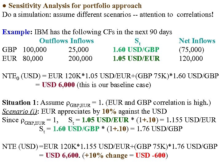● Sensitivity Analysis for portfolio approach Do a simulation: assume different scenarios attention to correlations! Example: IBM has the following CFs in the next 90 days Outflows Inflows St Net Inflows GBP 100, 000 25, 000 1. 60 USD/GBP (75, 000) EUR 80, 000 200, 000 1. 05 USD/EUR 120, 000 NTE 0 (USD) = EUR 120 K*1. 05 USD/EUR+(GBP 75 K)*1. 60 USD/GBP = USD 6, 000 (this is our baseline case) Situation 1: Assume GBP, EUR = 1. (EUR and GBP correlation is high. ) Scenario (i): EUR appreciates by 10% against the USD Since GBP, EUR = 1, St = 1. 05 USD/EUR * (1+. 10) = 1. 155 USD/EUR St = 1. 60 USD/GBP * (1+. 10) = 1. 76 USD/GBP NTE (USD) =EUR 120 K*1. 155 USD/EUR+(GBP 75 K)*1. 76 USD/GBP = USD 6, 600. (+10% change = USD -600)

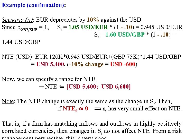Example (continuation): Scenario (ii): EUR depreciates by 10% against the USD Since GBP, EUR = 1, St = 1. 05 USD/EUR * (1 -. 10) = 0. 945 USD/EUR St = 1. 60 USD/GBP * (1 -. 10) = 1. 44 USD/GBP NTE (USD)=EUR 120 K*0. 945 USD/EUR+(GBP 75 K)*1. 44 USD/GBP = USD 5, 400. (-10% change = USD -600) Now, we can specify a range for NTE ∈ [USD 5, 400; USD 6, 600] Note: The NTE change is exactly the same as the change in St. Then, if NTE 0 ≈ 0 ⟹ st has very small effect on NTE. That is, if a firm has matching inflows and outflows in highly positively correlated currencies, then changes in St do not affect NTE. From a risk

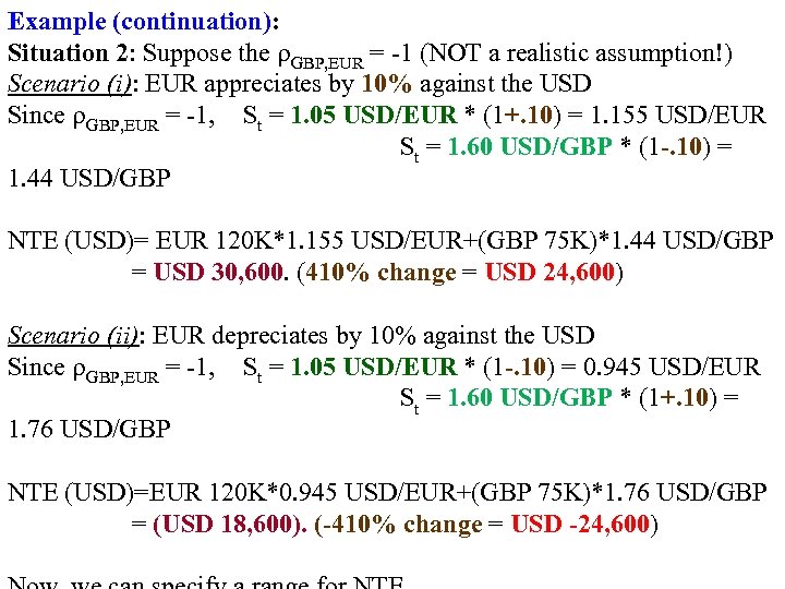Example (continuation): Situation 2: Suppose the GBP, EUR = 1 (NOT a realistic assumption!) Scenario (i): EUR appreciates by 10% against the USD Since GBP, EUR = 1, St = 1. 05 USD/EUR * (1+. 10) = 1. 155 USD/EUR St = 1. 60 USD/GBP * (1 -. 10) = 1. 44 USD/GBP NTE (USD)= EUR 120 K*1. 155 USD/EUR+(GBP 75 K)*1. 44 USD/GBP = USD 30, 600. (410% change = USD 24, 600) Scenario (ii): EUR depreciates by 10% against the USD Since GBP, EUR = 1, St = 1. 05 USD/EUR * (1 -. 10) = 0. 945 USD/EUR St = 1. 60 USD/GBP * (1+. 10) = 1. 76 USD/GBP NTE (USD)=EUR 120 K*0. 945 USD/EUR+(GBP 75 K)*1. 76 USD/GBP = (USD 18, 600). (-410% change = USD -24, 600)

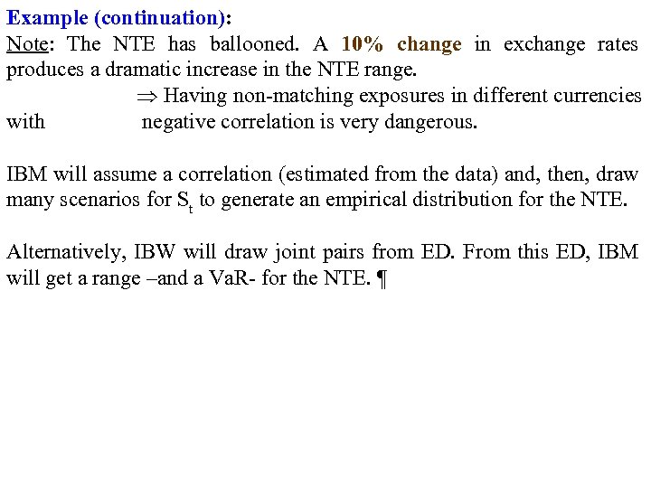Example (continuation): Note: The NTE has ballooned. A 10% change in exchange rates produces a dramatic increase in the NTE range. Having non matching exposures in different currencies with negative correlation is very dangerous. IBM will assume a correlation (estimated from the data) and, then, draw many scenarios for St to generate an empirical distribution for the NTE. Alternatively, IBW will draw joint pairs from ED. From this ED, IBM will get a range –and a Va. R for the NTE. ¶

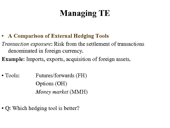Managing TE • A Comparison of External Hedging Tools Transaction exposure: Risk from the settlement of transactions denominated in foreign currency. Example: Imports, exports, acquisition of foreign assets. • Tools: Futures/forwards (FH) Options (OH) Money market (MMH) • Q: Which hedging tool is better?

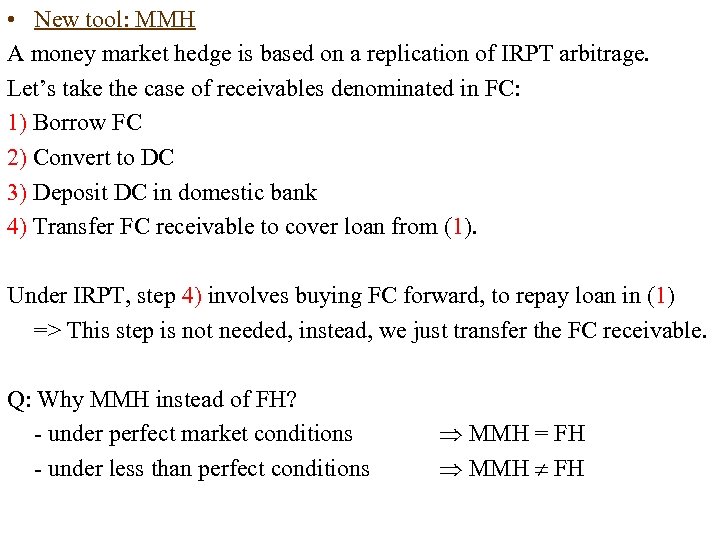• New tool: MMH A money market hedge is based on a replication of IRPT arbitrage. Let’s take the case of receivables denominated in FC: 1) Borrow FC 2) Convert to DC 3) Deposit DC in domestic bank 4) Transfer FC receivable to cover loan from (1). Under IRPT, step 4) involves buying FC forward, to repay loan in (1) => This step is not needed, instead, we just transfer the FC receivable. Q: Why MMH instead of FH? under perfect market conditions under less than perfect conditions MMH = FH MMH FH

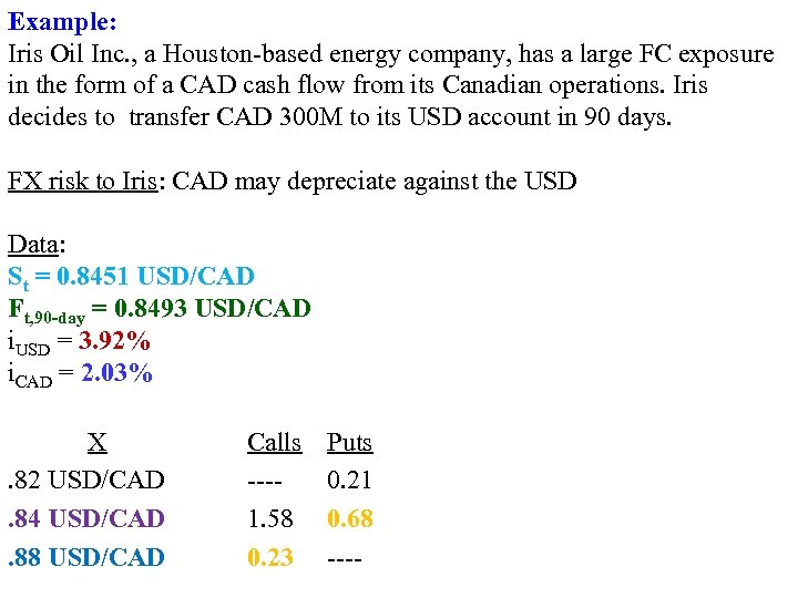Example: Iris Oil Inc. , a Houston based energy company, has a large FC exposure in the form of a CAD cash flow from its Canadian operations. Iris decides to transfer CAD 300 M to its USD account in 90 days. FX risk to Iris: CAD may depreciate against the USD Data: St = 0. 8451 USD/CAD Ft, 90 -day = 0. 8493 USD/CAD i. USD = 3. 92% i. CAD = 2. 03% X. 82 USD/CAD. 84 USD/CAD. 88 USD/CAD Calls 1. 58 0. 23 Puts 0. 21 0. 68

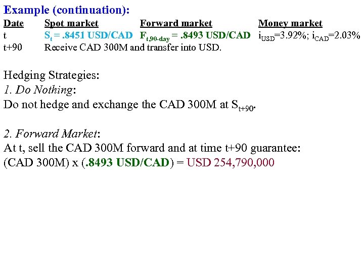Example (continuation): Date t t+90 Spot market Forward market Money market St =. 8451 USD/CAD Ft, 90 -day =. 8493 USD/CAD i. USD=3. 92%; i. CAD=2. 03% Receive CAD 300 M and transfer into USD. Hedging Strategies: 1. Do Nothing: Do not hedge and exchange the CAD 300 M at St+90. 2. Forward Market: At t, sell the CAD 300 M forward and at time t+90 guarantee: (CAD 300 M) x (. 8493 USD/CAD) = USD 254, 790, 000

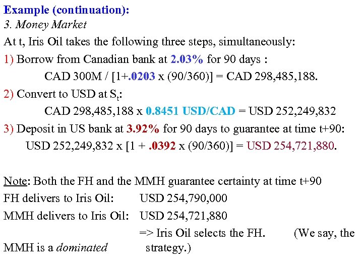Example (continuation): 3. Money Market At t, Iris Oil takes the following three steps, simultaneously: 1) Borrow from Canadian bank at 2. 03% for 90 days : CAD 300 M / [1+. 0203 x (90/360)] = CAD 298, 485, 188. 2) Convert to USD at St: CAD 298, 485, 188 x 0. 8451 USD/CAD = USD 252, 249, 832 3) Deposit in US bank at 3. 92% for 90 days to guarantee at time t+90: USD 252, 249, 832 x [1 +. 0392 x (90/360)] = USD 254, 721, 880. Note: Both the FH and the MMH guarantee certainty at time t+90 FH delivers to Iris Oil: USD 254, 790, 000 MMH delivers to Iris Oil: USD 254, 721, 880 => Iris Oil selects the FH. (We say, the MMH is a dominated strategy. )

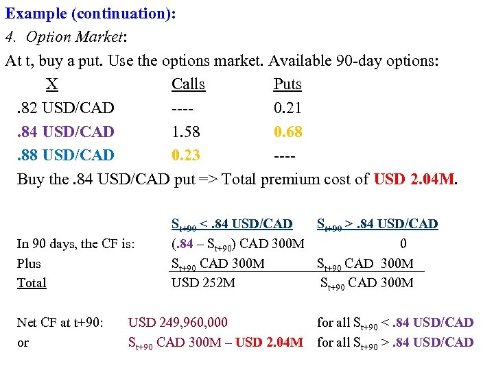Example (continuation): 4. Option Market: At t, buy a put. Use the options market. Available 90 day options: X Calls Puts. 82 USD/CAD 0. 21. 84 USD/CAD 1. 58 0. 68. 88 USD/CAD 0. 23 Buy the. 84 USD/CAD put => Total premium cost of USD 2. 04 M. In 90 days, the CF is: Plus Total Net CF at t+90: or St+90 <. 84 USD/CAD (. 84 – St+90) CAD 300 M St+90 CAD 300 M USD 252 M USD 249, 960, 000 St+90 CAD 300 M – USD 2. 04 M St+90 >. 84 USD/CAD 0 St+90 CAD 300 M for all St+90 <. 84 USD/CAD for all St+90 >. 84 USD/CAD

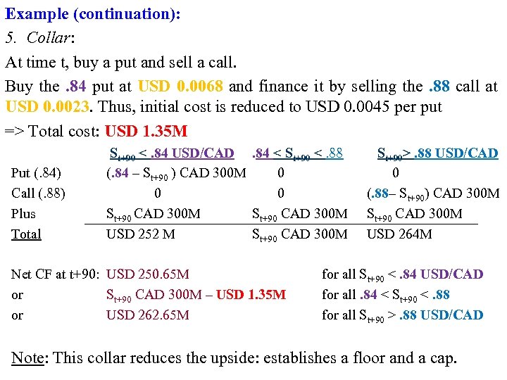Example (continuation): 5. Collar: At time t, buy a put and sell a call. Buy the. 84 put at USD 0. 0068 and finance it by selling the. 88 call at USD 0. 0023. Thus, initial cost is reduced to USD 0. 0045 per put => Total cost: USD 1. 35 M Put (. 84) Call (. 88) Plus Total St+90 <. 84 USD/CAD. 84 < St+90 <. 88 (. 84 – St+90 ) CAD 300 M 0 0 St+90 CAD 300 M USD 252 M St+90 CAD 300 M Net CF at t+90: USD 250. 65 M or St+90 CAD 300 M – USD 1. 35 M or USD 262. 65 M St+90>. 88 USD/CAD 0 (. 88– St+90) CAD 300 M St+90 CAD 300 M USD 264 M for all St+90 <. 84 USD/CAD for all. 84 < St+90 <. 88 for all St+90 >. 88 USD/CAD Note: This collar reduces the upside: establishes a floor and a cap.

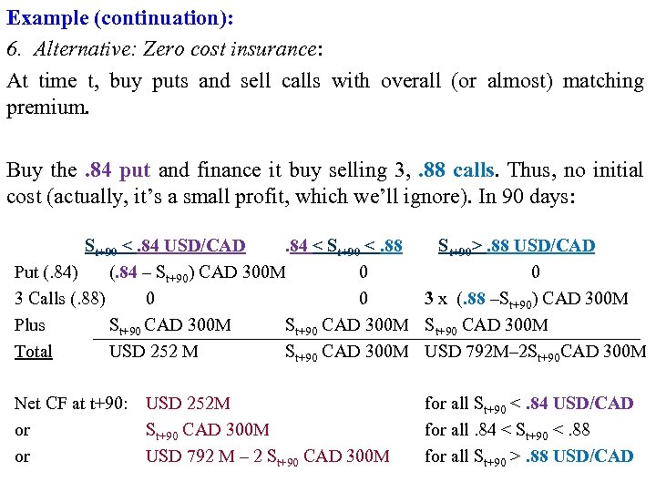Example (continuation): 6. Alternative: Zero cost insurance: At time t, buy puts and sell calls with overall (or almost) matching premium. Buy the. 84 put and finance it buy selling 3, . 88 calls. Thus, no initial cost (actually, it’s a small profit, which we’ll ignore). In 90 days: St+90 <. 84 USD/CAD. 84 < St+90 <. 88 Put (. 84) (. 84 – St+90) CAD 300 M 0 3 Calls (. 88) 0 0 Plus St+90 CAD 300 M Total USD 252 M St+90 CAD 300 M St+90>. 88 USD/CAD 0 3 x (. 88 –St+90) CAD 300 M St+90 CAD 300 M USD 792 M– 2 St+90 CAD 300 M Net CF at t+90: USD 252 M or St+90 CAD 300 M or USD 792 M – 2 St+90 CAD 300 M for all St+90 <. 84 USD/CAD for all. 84 < St+90 <. 88 for all St+90 >. 88 USD/CAD

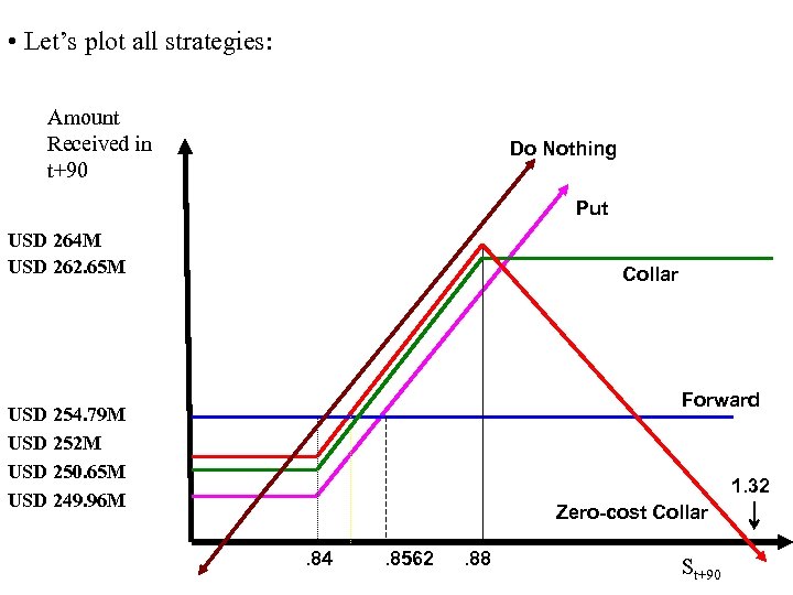• Let’s plot all strategies: Amount Received in t+90 Do Nothing Put USD 264 M USD 262. 65 M Collar Forward USD 254. 79 M USD 252 M USD 250. 65 M USD 249. 96 M 1. 32 Zero-cost Collar. 84 . 8562 . 88 St+90

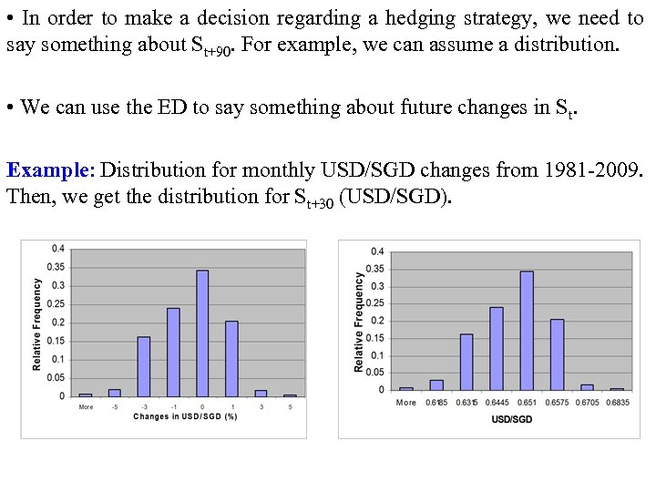• In order to make a decision regarding a hedging strategy, we need to say something about St+90. For example, we can assume a distribution. • We can use the ED to say something about future changes in St. Example: Distribution for monthly USD/SGD changes from 1981 2009. Then, we get the distribution for St+30 (USD/SGD).

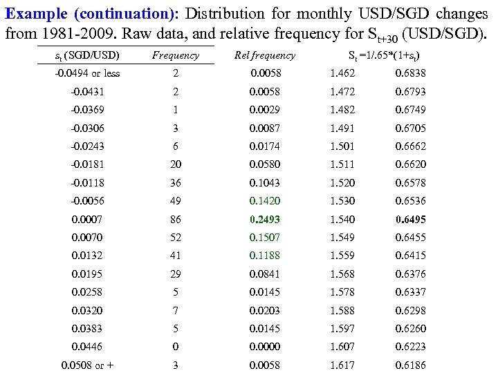Example (continuation): Distribution for monthly USD/SGD changes from 1981 2009. Raw data, and relative frequency for St+30 (USD/SGD). st (SGD/USD) Frequency Rel frequency St =1/. 65*(1+st) 0. 0494 or less 2 0. 0058 1. 462 0. 6838 0. 0431 2 0. 0058 1. 472 0. 6793 0. 0369 1 0. 0029 1. 482 0. 6749 0. 0306 3 0. 0087 1. 491 0. 6705 0. 0243 6 0. 0174 1. 501 0. 6662 0. 0181 20 0. 0580 1. 511 0. 6620 0. 0118 36 0. 1043 1. 520 0. 6578 0. 0056 49 0. 1420 1. 530 0. 6536 0. 0007 86 0. 2493 1. 540 0. 6495 0. 0070 52 0. 1507 1. 549 0. 6455 0. 0132 41 0. 1188 1. 559 0. 6415 0. 0195 29 0. 0841 1. 568 0. 6376 0. 0258 5 0. 0145 1. 578 0. 6337 0. 0320 7 0. 0203 1. 588 0. 6298 0. 0383 5 0. 0145 1. 597 0. 6260 0. 0446 0 0. 0000 1. 607 0. 6223 0. 0508 or + 3 0. 0058 1. 617 0. 6186

• Examples assuming an explicit distribution for St+T Example–Receivables: Evaluate (1) FH, (2) MMH, (3) OH and (4) NH. Cud Corp will receive SGD 500, 000 in 30 days. (SGD Receivable. ) Data: • St =. 6500 -. 6507 USD/SGD. • Ft, 30 =. 6510 -. 6519 USD/SGD. • 30 day interest rates: i. SGD: 2. 65% - 2. 75% & i. USD: 3. 20% - 3. 25% • A 30 day put option on SGD: X =. 65 USD/SGD and Pt= USD. 01. • Forecasted St+30: Possible Outcomes Probability USD. 63 18% USD. 64 24% USD. 65 34% USD. 66 21% USD. 68 3%

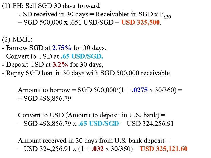(1) FH: Sell SGD 30 days forward USD received in 30 days = Receivables in SGD x Ft, 30 = SGD 500, 000 x. 651 USD/SGD = USD 325, 500. (2) MMH: Borrow SGD at 2. 75% for 30 days, Convert to USD at. 65 USD/SGD, Deposit USD at 3. 2% for 30 days, Repay SGD loan in 30 days with SGD 500, 000 receivable Amount to borrow = SGD 500, 000/(1 +. 0275 x 30/360) = = SGD 498, 856. 79 Convert to USD (Amount to deposit in U. S. bank) = = SGD 498, 856. 79 x. 65 USD/SGD = USD 324, 256. 91 Amount received in 30 days from U. S. bank deposit = = USD 324, 256. 91 x (1 +. 032 x 30/360) = USD 325, 121. 60

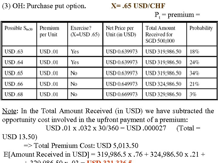(3) OH: Purchase put option. USD. 01 X=. 65 USD/CHF Pt = premium = Note: In the Total Amount Received (in USD) we have subtracted the opportunity cost involved in the upfront payment of a premium: USD. 01 x. 032 x 30/360 = USD. 000027 (Total = USD 13. 50) => Total Premium Cost: USD 5, 013. 50 E[Amount Received in USD] = 319, 986. 5 x. 76 + 324, 986. 50 x. 21 +

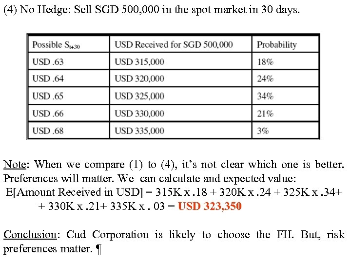(4) No Hedge: Sell SGD 500, 000 in the spot market in 30 days. Note: When we compare (1) to (4), it’s not clear which one is better. Preferences will matter. We can calculate and expected value: E[Amount Received in USD] = 315 K x. 18 + 320 K x. 24 + 325 K x. 34+ + 330 K x. 21+ 335 K x. 03 = USD 323, 350 Conclusion: Cud Corporation is likely to choose the FH. But, risk preferences matter. ¶

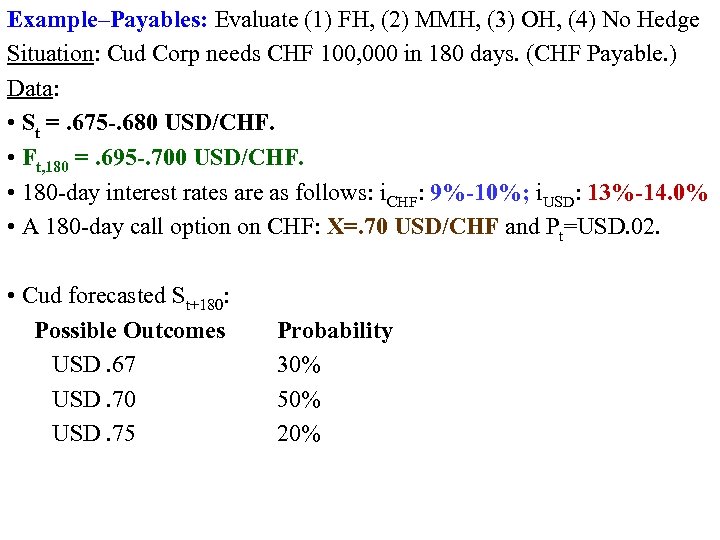Example–Payables: Evaluate (1) FH, (2) MMH, (3) OH, (4) No Hedge Situation: Cud Corp needs CHF 100, 000 in 180 days. (CHF Payable. ) Data: • St =. 675 -. 680 USD/CHF. • Ft, 180 =. 695 -. 700 USD/CHF. • 180 day interest rates are as follows: i. CHF: 9%-10%; i. USD: 13%-14. 0% • A 180 day call option on CHF: X=. 70 USD/CHF and Pt=USD. 02. • Cud forecasted St+180: Possible Outcomes USD. 67 USD. 70 USD. 75 Probability 30% 50% 20%

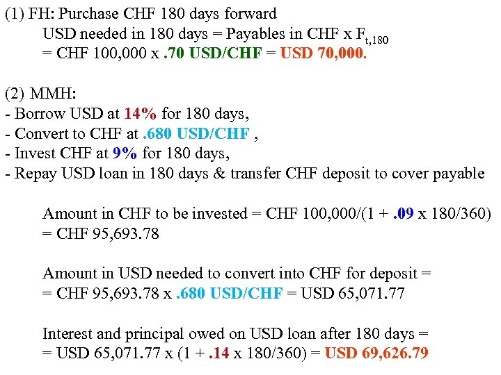(1) FH: Purchase CHF 180 days forward USD needed in 180 days = Payables in CHF x Ft, 180 = CHF 100, 000 x. 70 USD/CHF = USD 70, 000. (2) MMH: Borrow USD at 14% for 180 days, Convert to CHF at. 680 USD/CHF , Invest CHF at 9% for 180 days, Repay USD loan in 180 days & transfer CHF deposit to cover payable Amount in CHF to be invested = CHF 100, 000/(1 +. 09 x 180/360) = CHF 95, 693. 78 Amount in USD needed to convert into CHF for deposit = = CHF 95, 693. 78 x. 680 USD/CHF = USD 65, 071. 77 Interest and principal owed on USD loan after 180 days = = USD 65, 071. 77 x (1 +. 14 x 180/360) = USD 69, 626. 79

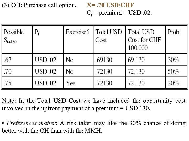(3) OH: Purchase call option. X=. 70 USD/CHF Ct = premium = USD. 02. Note: In the Total USD Cost we have included the opportunity cost involved in the upfront payment of a premium = USD 130. • Preferences matter: A risk taker may like the 30% chance of doing better with the OH than with the MMH.

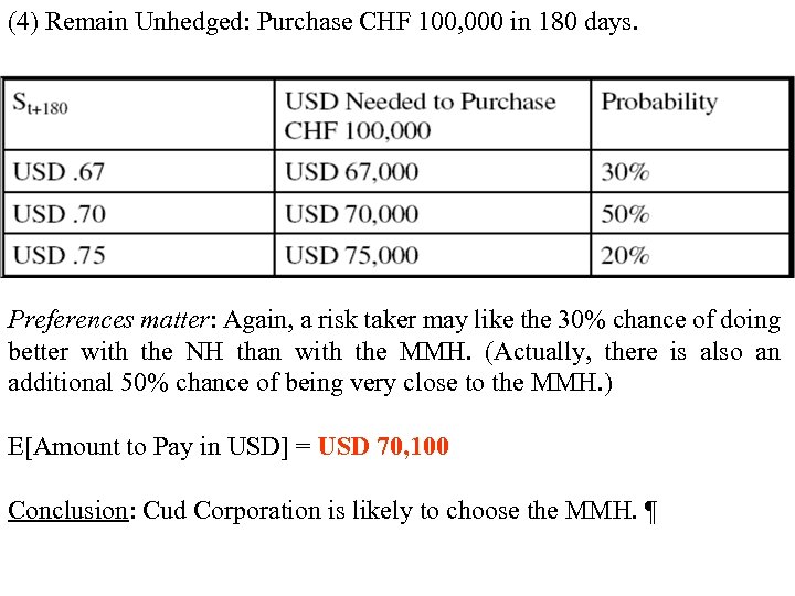(4) Remain Unhedged: Purchase CHF 100, 000 in 180 days. Preferences matter: Again, a risk taker may like the 30% chance of doing better with the NH than with the MMH. (Actually, there is also an additional 50% chance of being very close to the MMH. ) E[Amount to Pay in USD] = USD 70, 100 Conclusion: Cud Corporation is likely to choose the MMH. ¶

Internal Methods • These are hedging methods that do not involve financial instruments. • Risk Shifting Q: Can firms completely avoid exposure to exchange rate movements? A: Yes! By pricing all foreign transactions in the domestic currency. Example: Bossio Co. , a U. S. firm, sells naturally colored cotton. Asuni, a Japanese company, buys Bossio's cotton. Bossio Co. prices all exports in USD. ¶ => Currency risk is not eliminated. The foreign company bears it. • Problem with risk shifting: Reduces firm flexibility.

• Currency Risk Sharing Two parties can agree using a customized hedge contract to share the FX risk involved in the transaction. Example: Asuni buys cotton for USD 1 million from Bossio Co. Risk Sharing agreement: • If St [98 JPY/USD, 140 JPY/USD] transaction unchanged. (Asuni pays USD 1 M to Bossio Co. ) The range where the transaction is unchanged is called neutral zone. • If St < 98 JPY/USD or St > 140 JPY/USD both companies share the risk equally. Suppose that when Asuni has to pay Bossio Co. , St = 180 JPY/USD. The St used in settling the transaction is 160 JPY/USD (180 40/2). Asuni's final cost = JPY 160 million = USD 888, 889 < USD 1 M. ¶

• Leading and Lagging (L&L) Firms can reduce FX exposure by accelerating or decelerating the timing of payments that must be made in different currencies: leading or lagging the movement of funds. L&L is done between the parent company and its subsidiaries or between two subsidiaries. Example: Parent company: HAL (U. S. company). Subsidiaries: Mexico, Brazil, and Hong Kong. HAL Hong Kong's exposure is too large. HAL orders HAL Mexico and HAL Brazil to accelerate (lead) its payments to HAL Hong Kong. ¶ • L&L changes the assets or liabilities in one firm, with the reverse effect on the other firm. L&L changes balance sheet positions. Might be a good tool for achieving a hedged balance sheet position.

• Funds Adjustments Key to hedging: Match inflows and outflows denominated in the foreign currency. Chinese subsidiary in U. S. Italian subsidiary in U. S. has positive CFs in USD has negative CFs in USD Increase USD purchases Decrease CNY purchases Increase EUR purchases Decrease USD sales Increase CNY sales Decrease EUR sales Increase USD borrowing Reduce CNY borrowing Increase EUR borrowing Example: Japanese and German carmakers have plants in the U. S.

Translation Exposure Translation exposure: Risk from consolidating assets and liabilities measured in foreign currencies with those in the reporting currency. Assets and liabilities in a FC must be restated in terms of a DC. This translation follows rules set up by a parent firm's government, an accounting association (U. S. GAAP, or by the firm itself. Problem: The translation involves complex rules that sometimes reflect a compromise between historical and current exchange rates. => The translation might not end up with Assets=Liabilities.

• Examples of exchange rates used for translation: Historical rates may be used for some equity accounts, fixed assets, inventories. Current exchange rates are used for current assets, liabilities, expenses and income. Different exchange rates are used, imbalances will occur. • Key issue: what to do with the resulting imbalance? It is taken to either current income or equity reserves. Note: Translation exposure does not directly affect cash flows, but some firms are concerned about it because of its potential impact on reported consolidated earnings.

Measuring Translation Exposure There are several methods to translate foreign currency accounts into the reporting currency. Two methods that predominate: Temporal method (monetary/nonmonetary method) Current rate method Useful Terminology: Monetary: there is a date (maturity) attached to the asset or liability. Nonmonetary: items with no maturity (fixed assets, inventory). Three exchange rates can be used: S 0: Historical exchange rate. St: Current exchange rate at the date of balance. SAVERAGE: Average exchange rate for the period.

FASB #8 - Temporal Method (U. S. : used from 1976 1982) Premise: Historical cost accounting Translate nonmonetary assets at S 0, assets and liabilities use St Translate most income statements items at the SAVERAGE Translate shareholder equity at S 0 Bookkeeping exchange gains or losses are passed to the Income statement

FASB #52 - Current Rate Method (U. S. : used since 12/15/1982) Translate most amounts at St Income statement items are translated at S 0 or SAVERAGE Translate shareholder equity at S 0 Exchange gains or losses are not reflected in income statement rather accumulate in an adjustment account in stockholders' equity: Cumulative translation adjustment (CTA). Distinguished between functional currency (usually local currency) and reporting currency (currency in which the parent firm prepares its own financial statements) Exceptions to FASB #52 1. Accounts of subsidiaries whose operations are mostly with the parent use parent’s currency as functional currency, translate using temporal method. 2. Accounts of subsidiaries operating in hyperinflationary countries (over 100% over a three year period), functional currency must be the USD.

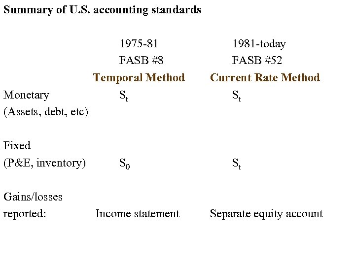Summary of U. S. accounting standards Monetary (Assets, debt, etc) Fixed (P&E, inventory) Gains/losses reported: 1975 81 FASB #8 Temporal Method St S 0 Income statement 1981 today FASB #52 Current Rate Method St St Separate equity account

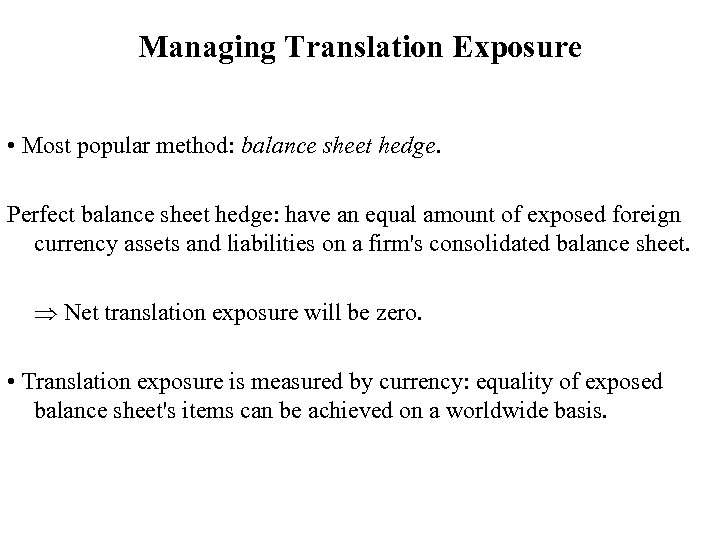Managing Translation Exposure • Most popular method: balance sheet hedge. Perfect balance sheet hedge: have an equal amount of exposed foreign currency assets and liabilities on a firm's consolidated balance sheet. Net translation exposure will be zero. • Translation exposure is measured by currency: equality of exposed balance sheet's items can be achieved on a worldwide basis.

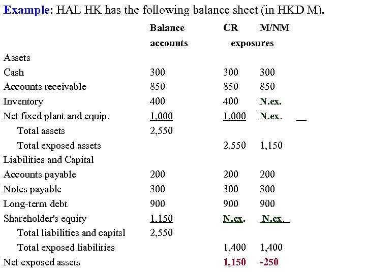Example: HAL HK has the following balance sheet (in HKD M). Balance accounts Assets Cash Accounts receivable Inventory Net fixed plant and equip. Total assets Total exposed assets Liabilities and Capital Accounts payable Notes payable Long term debt Shareholder's equity Total liabilities and capitsl Total exposed liabilities Net exposed assets CR M/NM exposures 300 850 400 1, 000 2, 550 300 850 400 1, 000 300 850 N. ex. 2, 550 1, 150 200 300 900 N. ex. 1, 400 1, 150 1, 400 -250 200 300 900 1, 150 2, 550

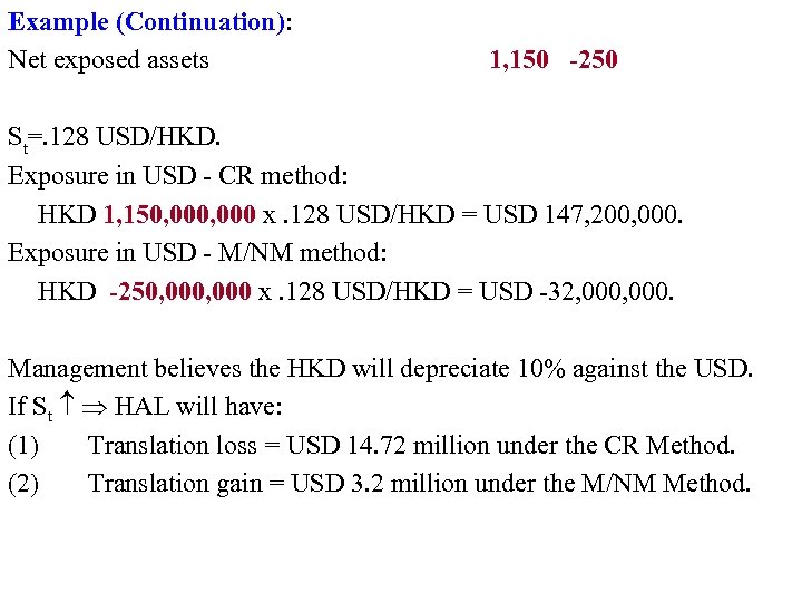Example (Continuation): Net exposed assets 1, 150 -250 St=. 128 USD/HKD. Exposure in USD CR method: HKD 1, 150, 000 x. 128 USD/HKD = USD 147, 200, 000. Exposure in USD M/NM method: HKD -250, 000 x. 128 USD/HKD = USD 32, 000. Management believes the HKD will depreciate 10% against the USD. If St HAL will have: (1) Translation loss = USD 14. 72 million under the CR Method. (2) Translation gain = USD 3. 2 million under the M/NM Method.

Example (Continuation): Note: Under the CR Method the loss will go to the CTA. Under the Temporal Method the gain will go to the income statement and increase earnings. HAL HK's functional currency is the HKD, HAL uses the CR Method. HAL wants to avoid translation exposure in HKD: HAL HK should borrow HKD 1, 150, 000, and then: (1) HAL HK could exchange the HKD for USD, or (2) HAL HK could transfer the borrowed HKD to HAL. ¶

Economic Exposure Economic exposure (EE): Risk associated with a change in the NPV of a firm's expected cash flows, due to an unexpected change in St. • Economic exposure is: Subjective. Difficult to measure. • We can use accounting data (changes in EAT) or financial/economic data (returns) to measure EE. Economists tend to like more economic data measures. • Note: Since St is very difficult to forecast, the actual change in St can be considered “unexpected. ”

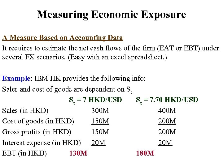Measuring Economic Exposure A Measure Based on Accounting Data It requires to estimate the net cash flows of the firm (EAT or EBT) under several FX scenarios. (Easy with an excel spreadsheet. ) Example: IBM HK provides the following info: Sales and cost of goods are dependent on St St = 7 HKD/USD St = 7. 70 HKD/USD Sales (in HKD) 300 M 400 M Cost of goods (in HKD) 150 M 200 M Gross profits (in HKD) 150 M 200 M Interest expense (in HKD) 20 M EBT (in HKD) 130 M 180 M

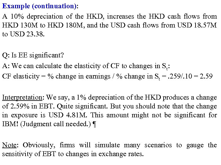Example (continuation): A 10% depreciation of the HKD, increases the HKD cash flows from HKD 130 M to HKD 180 M, and the USD cash flows from USD 18. 57 M to USD 23. 38. Q: Is EE significant? A: We can calculate the elasticity of CF to changes in St: CF elasticity = % change in earnings / % change in St =. 259/. 10 = 2. 59 Interpretation: We say, a 1% depreciation of the HKD produces a change of 2. 59% in EBT. Quite significant. But you should note that the change in exposure is USD 4. 81 M. This amount might not be significant for IBM! (Judgment call needed. ) ¶ Note: Obviously, firms will simulate many scenarios to gauge the sensitivity of EBT to changes in exchange rates.

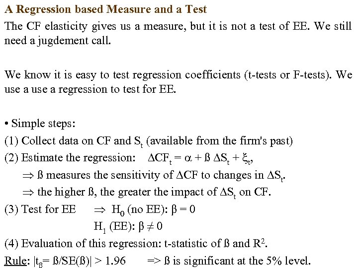A Regression based Measure and a Test The CF elasticity gives us a measure, but it is not a test of EE. We still need a jugdement call. We know it is easy to test regression coefficients (t tests or F tests). We use a regression to test for EE. • Simple steps: (1) Collect data on CF and St (available from the firm's past) (2) Estimate the regression: CFt = + ß St + t, ß measures the sensitivity of CF to changes in St. the higher ß, the greater the impact of St on CF. (3) Test for EE H 0 (no EE): β = 0 H 1 (EE): β ≠ 0 (4) Evaluation of this regression: t statistic of ß and R 2. Rule: |tβ= ß/SE(ß)| > 1. 96 => ß is significant at the 5% level.

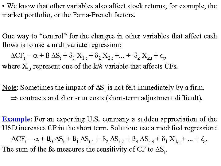• We know that other variables also affect stock returns, for example, the market portfolio, or the Fama French factors. One way to “control” for the changes in other variables that affect cash flows is to use a multivariate regression: CFt = + ß St + δ 1 X 1, t + δ 2 X 2, t +. . . + δk Xk, t + t, where Xi, t represent one of the kth variable that affects CFs. Note: Sometimes the impact of St is not felt immediately by a firm. contracts and short run costs (short term adjustment difficult). Example: For an exporting U. S. company a sudden appreciation of the USD increases CF in the short term. Solution: use a modified regression: CFt = + ß 0 St + ß 1 St 1 + ß 2 St 2 + ß 3 St 3 + δ 1 X 1, t +. . . + t. The sum of the ßs measures the sensitivity of CF to St.

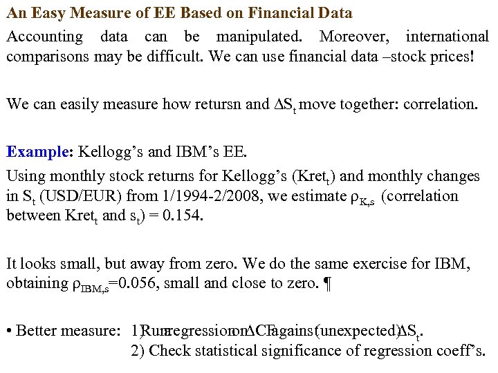An Easy Measure of EE Based on Financial Data Accounting data can be manipulated. Moreover, international comparisons may be difficult. We can use financial data –stock prices! We can easily measure how retursn and St move together: correlation. Example: Kellogg’s and IBM’s EE. Using monthly stock returns for Kellogg’s (Krett) and monthly changes in St (USD/EUR) from 1/1994 2/2008, we estimate ρK, s (correlation between Krett and st) = 0. 154. It looks small, but away from zero. We do the same exercise for IBM, obtaining ρIBM, s=0. 056, small and close to zero. ¶ • Better measure: 1) a Run regression CF on against (unexpected) t. S 2) Check statistical significance of regression coeff’s.

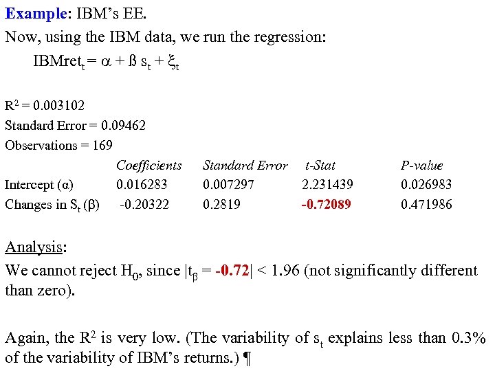Example: IBM’s EE. Now, using the IBM data, we run the regression: IBMrett = + ß st + t R 2 = 0. 003102 Standard Error = 0. 09462 Observations = 169 Coefficients Intercept (α) 0. 016283 Changes in St (β) 0. 20322 Standard Error 0. 007297 0. 2819 t-Stat 2. 231439 -0. 72089 P-value 0. 026983 0. 471986 Analysis: We cannot reject H 0, since |tβ = -0. 72| < 1. 96 (not significantly different than zero). Again, the R 2 is very low. (The variability of st explains less than 0. 3% of the variability of IBM’s returns. ) ¶

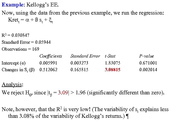Example: Kellogg’s EE. Now, using the data from the previous example, we run the regression: Krett = + ß st + t R 2 = 0. 030847 Standard Error = 0. 05944 Observations = 169 Coefficients Intercept (α) 0. 005991 Changes in St (β) 0. 512062 Standard Error 0. 003273 0. 165815 t-Stat 1. 83075 3. 08815 P-value 0. 671001 0. 002014 Analysis: We reject H 0, since |tβ = 3. 09| > 1. 96 (significantly different than zero). Note, however, that the R 2 is very low! (The variability of st explains less than 3. 08% of the variability of Kellogg’s returns. ) ¶

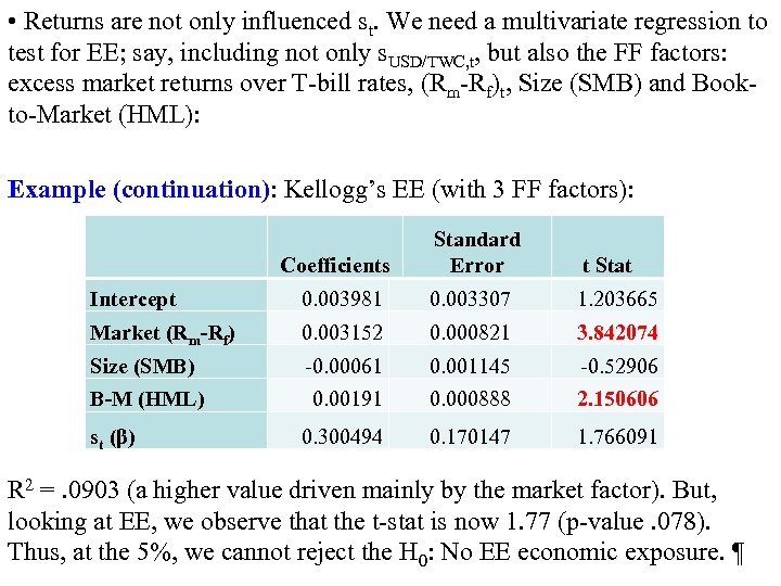• Returns are not only influenced st. We need a multivariate regression to test for EE; say, including not only s. USD/TWC, t, but also the FF factors: excess market returns over T bill rates, (Rm Rf)t, Size (SMB) and Book to Market (HML): Example (continuation): Kellogg’s EE (with 3 FF factors): Coefficients Standard Error t Stat Intercept 0. 003981 0. 003307 1. 203665 Market (Rm-Rf) 0. 003152 0. 000821 3. 842074 Size (SMB) 0. 00061 0. 001145 0. 52906 B-M (HML) 0. 00191 0. 000888 2. 150606 0. 300494 0. 170147 1. 766091 st (β) R 2 =. 0903 (a higher value driven mainly by the market factor). But, looking at EE, we observe that the t stat is now 1. 77 (p value. 078). Thus, at the 5%, we cannot reject the H 0: No EE economic exposure. ¶

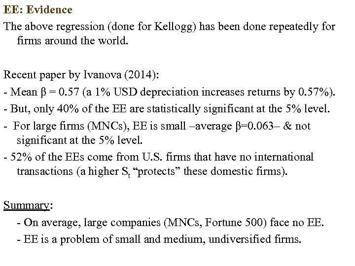EE: Evidence The above regression (done for Kellogg) has been done repeatedly for firms around the world. Recent paper by Ivanova (2014): Mean β = 0. 57 (a 1% USD depreciation increases returns by 0. 57%). But, only 40% of the EE are statistically significant at the 5% level. For large firms (MNCs), EE is small –average β=0. 063– & not significant at the 5% level. 52% of the EEs come from U. S. firms that have no international transactions (a higher St “protects” these domestic firms). Summary: On average, large companies (MNCs, Fortune 500) face no EE. EE is a problem of small and medium, undiversified firms.

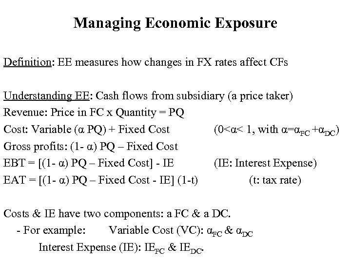Managing Economic Exposure Definition: EE measures how changes in FX rates affect CFs Understanding EE: Cash flows from subsidiary (a price taker) Revenue: Price in FC x Quantity = PQ Cost: Variable (α PQ) + Fixed Cost (0<α< 1, with α=αFC +αDC) Gross profits: (1 α) PQ – Fixed Cost EBT = [(1 α) PQ – Fixed Cost] IE (IE: Interest Expense) EAT = [(1 α) PQ – Fixed Cost IE] (1 t) (t: tax rate) Costs & IE have two components: a FC & a DC. For example: Variable Cost (VC): αFC & αDC Interest Expense (IE): IEFC & IEDC.

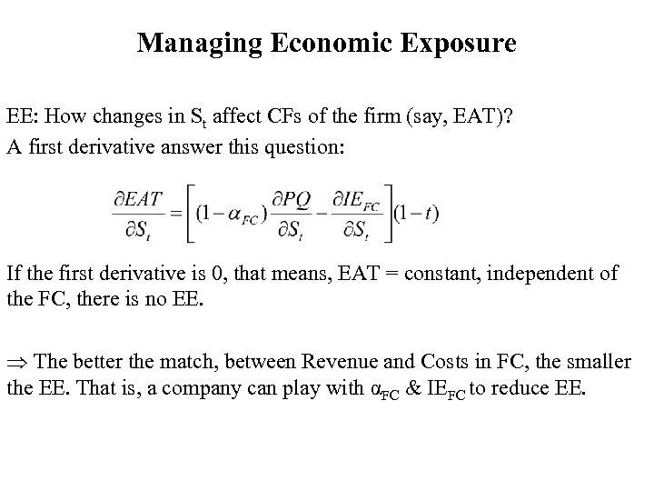Managing Economic Exposure EE: How changes in St affect CFs of the firm (say, EAT)? A first derivative answer this question: If the first derivative is 0, that means, EAT = constant, independent of the FC, there is no EE. The better the match, between Revenue and Costs in FC, the smaller the EE. That is, a company can play with αFC & IEFC to reduce EE.

Managing Economic Exposure • Matching Inflows and Outflows Q: How can a firm get a good match? Play with αFC to establish a manageable EE. For example, if Fixed Costs and IE are small relative to VC, then, the bigger αFC, the smaller the exposed CF (EAT) to changes in S. t When a firm restructures operations (shift expenses to FC, by increasing αFC) to reduce EE, we say a firm is doing operational hedging.

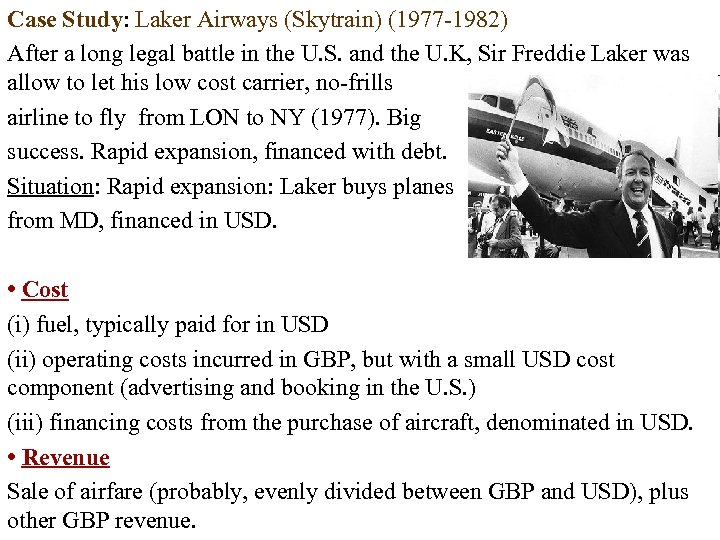Case Study: Laker Airways (Skytrain) (1977 1982) After a long legal battle in the U. S. and the U. K, Sir Freddie Laker was allow to let his low cost carrier, no frills airline to fly from LON to NY (1977). Big success. Rapid expansion, financed with debt. Situation: Rapid expansion: Laker buys planes from MD, financed in USD. • Cost (i) fuel, typically paid for in USD (ii) operating costs incurred in GBP, but with a small USD cost component (advertising and booking in the U. S. ) (iii) financing costs from the purchase of aircraft, denominated in USD. • Revenue Sale of airfare (probably, evenly divided between GBP and USD), plus other GBP revenue.

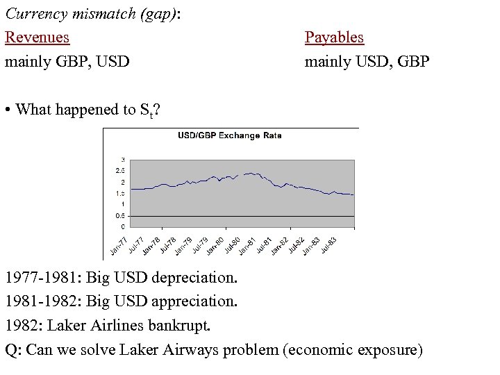Currency mismatch (gap): Revenues mainly GBP, USD Payables mainly USD, GBP • What happened to St? 1977 1981: Big USD depreciation. 1981 1982: Big USD appreciation. 1982: Laker Airlines bankrupt. Q: Can we solve Laker Airways problem (economic exposure)

• Solutions to Laker Airways problem (economic exposure): Increase sales in US Increase IE in GBP (borrow more in the UK) Transfer cost out to GBP/Shift expenses to GBP (αDC↑ /αFC ↓) Diversification • Severe problems show up when there is a currency gap (= Inflows in FC Ouflows in FC). • Very simple approach to managing EE: Minimize currency gaps. match inflows in FC and outflows in FC as much as possible. • European and Japanese car makers have been matching inflows and outflows by moving production to the U. S. But, not all companies can avoid currency gaps: Importing and Exporting companies will always be operationally exposed.

Q: Why Operational Hedging? Financial hedging –i. e. , with FX derivative instruments– is inexpensive, but tends to be short term, liquid only for short term maturities. Operational hedging is more expensive (increasing αFC by building a plant, expansion of offices, etc. ) but a long term instrument. A different view: Financial hedging only covers FX risk (St through P), but not the risk associated with sales in the foreign country (Q risk). For example, if the foreign country enters into a recession, Q will go down, but not necessarily St. An operational hedge works better to cover Q risk. From this view, financial hedging does not work very well if the correlation between price in FC (P) and quantity sold (Q) is low. On the other hand, if Corr(P, Q) is high, financial hedging will be OK.

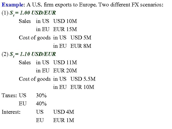Example: A U. S. firm exports to Europe. Two different FX scenarios: (1) St = 1. 00 USD/EUR Sales in US USD 10 M in EU EUR 15 M Cost of goods in US USD 5 M in EU EUR 8 M (2) St = 1. 10 USD/EUR Sales in US USD 11 M in EU EUR 20 M Cost of goods in US USD 5. 5 M in EU EUR 10 M Taxes: US 30% EU 40% Interest: US USD 4 M EU EUR 1 M

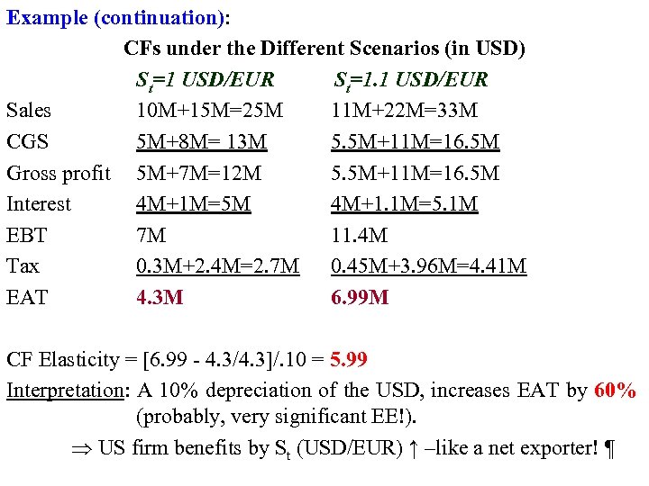Example (continuation): CFs under the Different Scenarios (in USD) St=1 USD/EUR St=1. 1 USD/EUR Sales 10 M+15 M=25 M 11 M+22 M=33 M CGS 5 M+8 M= 13 M 5. 5 M+11 M=16. 5 M Gross profit 5 M+7 M=12 M 5. 5 M+11 M=16. 5 M Interest 4 M+1 M=5 M 4 M+1. 1 M=5. 1 M EBT 7 M 11. 4 M Tax 0. 3 M+2. 4 M=2. 7 M 0. 45 M+3. 96 M=4. 41 M EAT 4. 3 M 6. 99 M CF Elasticity = [6. 99 4. 3/4. 3]/. 10 = 5. 99 Interpretation: A 10% depreciation of the USD, increases EAT by 60% (probably, very significant EE!). US firm benefits by St (USD/EUR) ↑ –like a net exporter! ¶

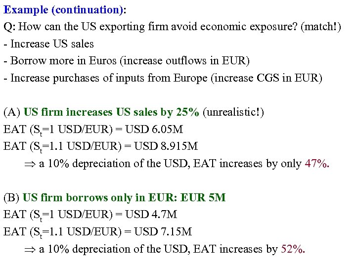Example (continuation): Q: How can the US exporting firm avoid economic exposure? (match!) Increase US sales Borrow more in Euros (increase outflows in EUR) Increase purchases of inputs from Europe (increase CGS in EUR) (A) US firm increases US sales by 25% (unrealistic!) EAT (St=1 USD/EUR) = USD 6. 05 M EAT (St=1. 1 USD/EUR) = USD 8. 915 M a 10% depreciation of the USD, EAT increases by only 47%. (B) US firm borrows only in EUR: EUR 5 M EAT (St=1 USD/EUR) = USD 4. 7 M EAT (St=1. 1 USD/EUR) = USD 7. 15 M a 10% depreciation of the USD, EAT increases by 52%.

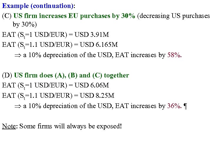Example (continuation): (C) US firm increases EU purchases by 30% (decreasing US purchases by 30%) EAT (St=1 USD/EUR) = USD 3. 91 M EAT (St=1. 1 USD/EUR) = USD 6. 165 M a 10% depreciation of the USD, EAT increases by 58%. (D) US firm does (A), (B) and (C) together EAT (St=1 USD/EUR) = USD 6. 06 M EAT (St=1. 1 USD/EUR) = USD 8. 25 M a 10% depreciation of the USD, EAT increases by 36%. ¶ Note: Some firms will always be exposed!

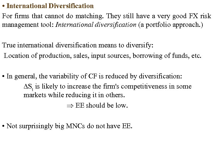• International Diversification For firms that cannot do matching. They still have a very good FX risk management tool: International diversification (a portfolio approach. ) True international diversification means to diversify: Location of production, sales, input sources, borrowing of funds, etc. • In general, the variability of CF is reduced by diversification: St is likely to increase the firm's competitiveness in some markets while reducing it in others. EE should be low. • Not surprisingly big MNCs do not have EE.

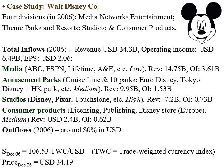• Case Study: Walt Disney Co. Four divisions (in 2006): Media Networks Entertainment; Theme Parks and Resorts; Studios; & Consumer Products. Total Inflows (2006) Revenue USD 34. 3 B, Operating income: USD 6. 49 B, EPS: USD 2. 06: Media (ABC, ESPN, Lifetime, A&E, etc. Low). Rev: 14. 75 B, OI: 3. 61 B Amusement Parks (Cruise Line & 10 parks: Euro Disney, Tokyo Disney + HK park, etc. Medium). Rev: 9. 95 B, OI: 1. 53 B Studios (Disney, Pixar, Touchstone, etc. High). Rev: 7. 2 B, OI: 0. 73 B Consumer products (Licensing, Publishing, Disney store (Europe). Medium) Rev: USD 2. 4 B, OI: 0. 62 B Outflows (2006) – around 80% in USD SDec 06 = 106. 53 TWC/USD (TWC = Trade weighted currency index) Price. Dec 06 = USD 34. 19

• Case Study: Walt Disney Co. UPDATE (2006 -2013): DIS bought Marvel (USD 4 B) in 2009 and Lucasfilm (USD 4 B) in 2012. DIS introduced a new division: Interactive Media (Kaboosee. com, Baby. Zone. com, Playdom (social gaming), etc. ) DIS ordered two new cruises with 50% more capacity each in 2011. Shangai theme park to be opened in 2016. Q: Economic Exposure? Yes. Probably: Medium • Check intuition: Calculate a pseudo elasticity; using 2006 2013 data: 13 06 Change in OI = USD 10. 72 B – USD 6. 49 = USD 4. 23 B (65. 18%) 13 06 DIS Stock Return = 65. 30/34. 19 – 1 = 111. 32% 13 06 st = 106. 53/101. 923 1 = 0. 05725 (or 5. 73% depreciation of the USD, as direct quote)

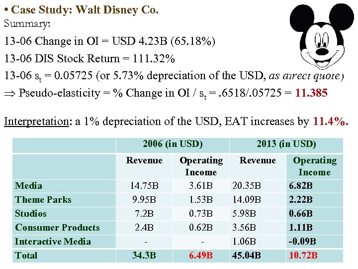• Case Study: Walt Disney Co. Summary: 13 06 Change in OI = USD 4. 23 B (65. 18%) 13 06 DIS Stock Return = 111. 32% 13 06 st = 0. 05725 (or 5. 73% depreciation of the USD, as direct quote) Pseudo elasticity = % Change in OI / st =. 6518/. 05725 = 11. 385 Interpretation: a 1% depreciation of the USD, EAT increases by 11. 4%. Media Theme Parks Studios Consumer Products Interactive Media Total 2006 (in USD) Revenue 14. 75 B 9. 95 B 7. 2 B 2. 4 B 34. 3 B Operating Income 3. 61 B 1. 53 B 0. 73 B 0. 62 B 6. 49 B 2013 (in USD) Revenue 20. 35 B 14. 09 B 5. 98 B 3. 56 B 1. 06 B 45. 04 B Operating Income 6. 82 B 2. 22 B 0. 66 B 1. 11 B -0. 09 B 10. 72 B

• Case Study: Walt Disney Co. If stock market numbers are more trusted, recalculate pseudo elasticity as: DIS Stock Return/st = 1. 1132/. 05725 = 19. 45 • According to these elasticities, DIS behaves like a net exporter: St (USD/TW) ↑ CFs ↑. • Q: Is this pseudo elasticity informative? Is St the only variable changing from 2006 to 2013? A: No! For example, DIS added assets, then more revenue and OI is expected. We need to be careful with these numbers. We need to “control” for these changes, to isolate the effect of st.

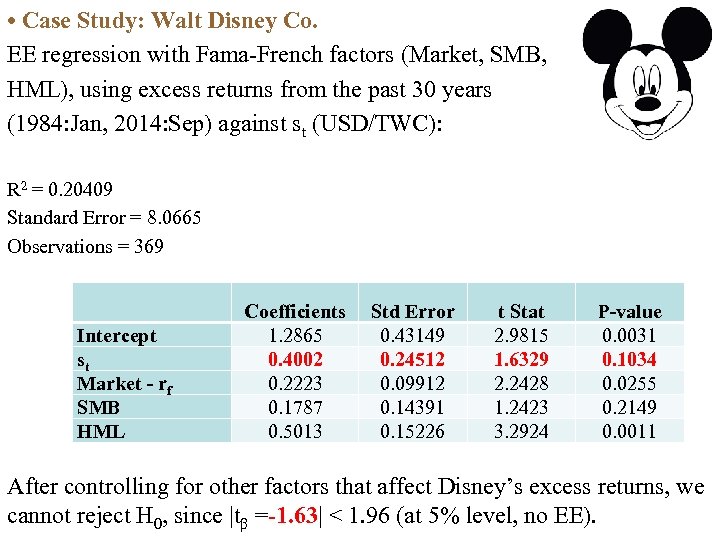• Case Study: Walt Disney Co. EE regression with Fama French factors (Market, SMB, HML), using excess returns from the past 30 years (1984: Jan, 2014: Sep) against st (USD/TWC): R 2 = 0. 20409 Standard Error = 8. 0665 Observations = 369 Intercept st Market - rf SMB HML Coefficients 1. 2865 0. 4002 0. 2223 0. 1787 0. 5013 Std Error 0. 43149 0. 24512 0. 09912 0. 14391 0. 15226 t Stat 2. 9815 1. 6329 2. 2428 1. 2423 3. 2924 P-value 0. 0031 0. 1034 0. 0255 0. 2149 0. 0011 After controlling for other factors that affect Disney’s excess returns, we cannot reject H 0, since |tβ = 1. 63| < 1. 96 (at 5% level, no EE).

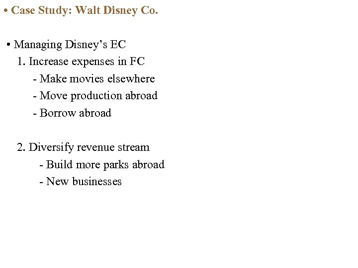• Case Study: Walt Disney Co. • Managing Disney’s EC 1. Increase expenses in FC Make movies elsewhere Move production abroad Borrow abroad 2. Diversify revenue stream Build more parks abroad New businesses

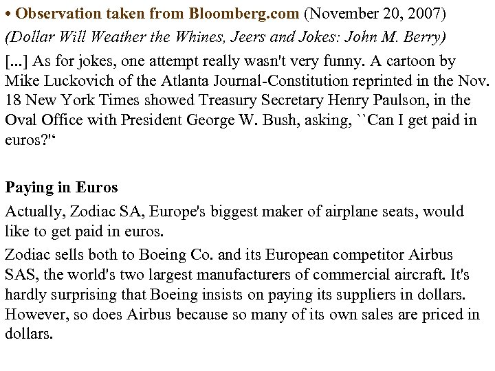• Observation taken from Bloomberg. com (November 20, 2007) (Dollar Will Weather the Whines, Jeers and Jokes: John M. Berry) [. . . ] As for jokes, one attempt really wasn't very funny. A cartoon by Mike Luckovich of the Atlanta Journal Constitution reprinted in the Nov. 18 New York Times showed Treasury Secretary Henry Paulson, in the Oval Office with President George W. Bush, asking, ``Can I get paid in euros? '‘ Paying in Euros Actually, Zodiac SA, Europe's biggest maker of airplane seats, would like to get paid in euros. Zodiac sells both to Boeing Co. and its European competitor Airbus SAS, the world's two largest manufacturers of commercial aircraft. It's hardly surprising that Boeing insists on paying its suppliers in dollars. However, so does Airbus because so many of its own sales are priced in dollars.

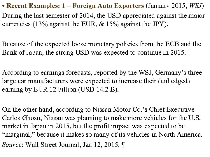• Recent Examples: 1 – Foreign Auto Exporters (January 2015, WSJ) During the last semester of 2014, the USD appreciated against the major currencies (13% against the EUR, & 15% against the JPY). Because of the expected loose monetary policies from the ECB and the Bank of Japan, the strong USD was expected to continue in 2015. According to earnings forecasts, reported by the WSJ, Germany’s three large car manufacturers were expected to increase their (unhedged) earning by EUR 12 billion (USD 14. 2 B). On the other hand, according to Nissan Motor Co. ’s Chief Executive Carlos Ghosn, Nissan was planning to make more vehicles for the U. S. market in Japan in 2015, but the profit impact was expected to be “marginal, ” because it makes so many of its vehicles in North America. Source: Wall Street Journal, Jan 12, 2015. ¶

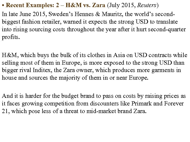• Recent Examples: 2 – H&M vs. Zara (July 2015, Reuters) In late June 2015, Sweden’s Hennes & Mauritz, the world’s second biggest fashion retailer, warned it expects the strong USD to translate into rising sourcing costs throughout the year after it hurt second quarter profits. H&M, which buys the bulk of its clothes in Asia on USD contracts while selling most of them in Europe, is more exposed to the strong USD than bigger rival Inditex, the Zara owner, which produces more garments in house and sources the majority of them in or near Europe. And it is harder for the budget brand to pass on costs by raising prices as it faces growing competition from discounters like Primark and Forever 21, which pose less of a threat to mid market brand Zara.

• Recent Examples: Conclusions Better match lower EE. Zara has a better match between FC receivables and FC costs than H&M, and, thus, lower EE. Similar situation applies to Nissan relative to the big 3 German firms (confirmed by Nissan’s executive Ghosn: Nissan’s has a very good match in USD, creating a very low EE).

Should a Firm Hedge? • Fundamental question: Does hedging add value to a firm? There are two views: (1) Modigliani Miller Theorem (MMT): (2) MMT assumptions are violated hedging adds no value. hedging adds value. The MMT depends on a set of assumptions: MM requires that a firm operates in perfect markets.

• Hedging is Irrelevant: The MMT Intuition: What is the value of your car? Example 1: You bought a last year car using a bank loan. Q: Is the value of your car affected by the loan you took to pay for it? • MMT provides a similar story to value a firm. Firms make money if they make good investments. The financing source of those good investments is irrelevant. Different mechanisms of financing will determine how the cash flows are divided among shareholders or bondholders. • Hedging works like insurance. Example 2: You bought insurance for your car. Q: Is the value of your car affected by the insurance you took?

• MMT's hedging implications. If the methods of financing and the character of financial risks do not matter, managing them is not important: Hedging should not add any value to a firm. • Hedging increases the portfolio of the firm. But, hedging is not free: Hedging might reduce the value of a firm. • Another result: Investors can hedge (diversify) by themselves. Example: Ms. Sternin holds shares of a U. S. exporting firm and shares of a U. S. importing firm. Ms. Sternin's portfolio is hedged. A USD depreciation will negatively affect the importing firm and will positively affect the exporting firm. Hedging at the firm level since it is not free will negatively affect the value of Ms. Sternin portfolio. ¶

• Hedging Adds Value Key: MMT assumptions are violated in the "real world. “ (1) Investors might not be able to replicate an optimal hedge Sometimes firms can do a better job at hedging than individuals. Example: Investors might not be big enough have enough information (2) Hedging as a tool to reduce the risk of bankruptcy If cash flows are very volatile, a firm might be faced with the problem of needing cash to meet its debt obligations. Conclusion: Firms with little debt or with good access to credit have no need to hedge. Note: Under this view, large corporations may be wasting their capital.

(3) Hedging as a tool to reduce investment uncertainty Firms should hedge to ensure they always have sufficient cash flow to fund their planned investment plan. For example, an exporting firm might have cash flows problems in periods when the USD appreciates. Example: Merk, a U. S. pharmaceutical firm, has used derivatives to ensure that investment (R&D) plans can always be financed. ¶ (4) Hedging as a bank loan requirement. Stable CFs to get bank financing. (5) Herding “Everybody else is hedging. I should hedge too; otherwise, I may not look good. ”

• Do U. S. Firms Hedge? From a survey of the largest 250 U. S. MNCs, taken in (2001): (1) Most of the MNCs in the survey understood translation, transactions, and economic exposure completely or substantially. (2) A large percentage (32% 44%) hedged themselves substantially or partially. However, a larger percentage did not cover themselves at all against transactions and economic exposure. (3) A significant percentage of the firms' hedging decisions depended on future FX fluctuations. (4) Over 25% of firms indicated that they used the forward hedge. (5) The majority of the firms surveyed have a better understanding of transactions and translation exposure than of economic exposure.

• Canadian Evidence The Bank of Canada conducts an annual survey of FX hedging. The main findings from the 2011 survey are: • Companies hedge approximately 50% of their FX risk. • Usually, hedging is for maturities of six months or less. • Use of FX options is relatively low, mainly because of accounting rules and restrictions imposed by treasury mandate, rules or policies. • Growing tendency for banks to pass down the cost of credit (credit valuation adjustment) to their clients. • Exporters were reluctant to hedge because they were anticipating that the CAD would depreciate. On the other hand, importers increased both their hedging ratio and duration.

Joke: Talking About Accounting Never trust your Accountant or Stockbroker - The Franciscan The Godfather, accompanied by his stockbroker, walks into a room to meet with his accountant. The Godfather asks the accountant, “Where’s the three million bucks you embezzled from me? ” The accountant doesn’t answer. The Godfather asks again, “Where’s the three million bucks you embezzled from me? ” The stockbroker interrupts, “Sir, the man is a deaf mute and cannot understand you, but I can interpret for you. ” The Godfather says, “Well, ask him where the @#!* money is. ” The stockbroker, using sign language, asks the accountant where three million dollars is. The accountant signs back, “I don’t know what you’re talking about. ” The stockbroker interprets to the Godfather, “He doesn’t know what you’re talking about. ” The Godfather pulls out a pistol, puts it to the temple of the accountant, cocks the trigger and says, “Ask him again where the @#!* money is!” The stockbroker signs to the accountant, “He wants to know where it is!” The accountant signs back, “Okay! The money’s hidden in a suitcase behind the shed in my backyard!” The Godfather says, “Well, what did he say? ” The stockbroker interprets to the Godfather, “He says that you don’t have the guts to pull the trigger. ”