Functions Limits and the Derivative 2 Functions

Functions, Limits, and the Derivative 2 • Functions and Their Graphs • The Algebra of Functions • Functions and Mathematical Models • Limits • One-Sided Limits and Continuity • The Derivative

Function A rule that assigns to each element in a set A (the domain), one and only one element in a set B (the range) Domain A mapping 1 3 -4 Range B -1 1 -6

Function Ø A function is a rule that assigns to each object in a set A exactly one object in a set B. Ø The set A is called the domain of the function, and the set of assigned objects in B is called the range.

Function, or not? YES NO NO

Function Notation is a function, with values of x as the domain and values of y as the range. We write in place of y. This is read “f of x. ” So NOTE: It is not f times x

Ø To be convenient, we represent a functional relationship by an equation Ø In this context, x and y are called variable, furthermore, we refer to y as the dependent variable and to x as the independent variable. For instant, the function representation Ø Noted that x and y can be substituted by other letters. For example, the above function can be represented by

Function Notation Example Solution Plug in – 2

Function that describes tabular data Table 1. 1 Average Tuition and Fees for 4 -Year Private Colleges Academic Year Ending in 1973 1978 1983 1988 1993 1998 2003 Period n 1 2 3 4 5 6 7 Tuition and Fees $1, 898 $2, 700 $4, 639 $7, 048 $10, 448 $13, 785 $18, 273

Ø So how can we use functional notation to describe this kind of data that is listed in Table 1. 1? Ø We can describe this data as a function f defined by the rule Thus, Ø Noted that the domain of f is the set of integers Ø What is the range of f ?

Piecewise-defined function Ø A piecewise-defined function is such a function that is often defined using more than one formula, where each individual formula describes the function on a subset of the domain. Ø Here is an example of such a function

Example 1 Find f(-1/2), f(1), and f(2), where the piecewise-defined function f(x) is given at the foregoing slide. Solution: Since find satisfies x<1, use the top part of the formula to However, x=1 and x=2 satisfy x≥ 1, so f(1) and f(2) are both found by using the bottom part of the formula: and

Domain Convention Ø We assume the domain of f to be the set of all numbers for which f(x) is defined (as a real number). Ø We refer to this as the natural domain of f. In general, there are two situations where a number is not in the domain of a function: 1) division by 0 2) The even number root of a negative number

Domain of a Function Ex 1. Find the domain of Since division by zero is undefined we must The domain can be expressed as the intervals

Domain of a Function Ex 2. Find the domain of Since the square root of a negative number is undefined we must have The domain can be expressed as the interval

Example 3 Find the domain and range of each of these functions a. b. Solution: a. Since division by any number other than 0 is possible, the domain of f is the set of all numbers except 3. The range of f is the set of all numbers y except 0, since for any y≠ 0, there is an x such that ; in particular, . b. Since negative numbers do not have real fourth roots, so the domain of g is the set of all numbers u such as u≥-2. The range of g is the set of all nonnegative numbers.

Graph of a Function The graph of a function is the set of all points (x, y) such that x is in the domain of f and y = f (x). Given the graph of y = f (x), find f (1). y f (1) = 2 (1, 2) x

Graph of a Function Ø The graph of a function f consists of all points (x, y) where x is in the domain of f and y=f(x), that is, all points of the form (x, f(x)). Ø Rectangular coordinate system, Horizontal axis, vertical axis. Ø The below example shows that the function can be sketched by plotting a few points. x -3 -2 -1 0 1 2 3 4 f(x) -10 -4 0 2 2 0 -4 -10

Parabolas Ø Parabolas: The graph of as long as A≠ 0. Ø All parabolas have a “U shape” and the parabola opens up if A>0 and down if A<0. Ø The “peak” or “valley” of the parabola is called its vertex, and it always occurs where

Intersections of Graphs Ø Sometimes it is necessary to determine when two functions are equal. For example, an economist may wish to compute the market price at which the consumer demand for a commodity will be equal to supply. Ø

The Vertical Line Test: The graph of a function can be crossed at most once by any vertical line. Function Not a Function It is crossed more than once.

The Vertical Line Test: A curve is the graph of a function if and only if no vertical line intersects the curve more than once.

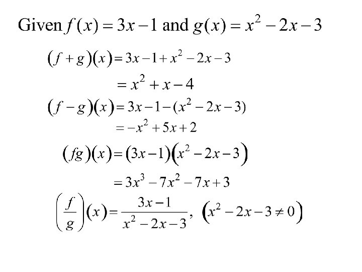
Algebra of Functions Domain: Domain of f intersected with the domain of g with the exclusion of all values of x, such that g(x) = 0.

Application Example (Functions ) Ø The total revenue is given by the product R(x)=(number of items sold)(price per item) =xp=x. D(x) Ø If C(x) is the total cost of producing the x units, the profit is given by the function P(x)=R(x)-C(x)=x. D(x)-C(x)

Example Market research indicates that consumers will buy x thousand units of a particular kind of coffee maker when the unit price is dollars. The cost of producing the x thousand units is thousand dollars. a. What are the revenue and profit functions, R(x) and P(x), for this production process? b. For what values of x is production of the coffee makers profitable?

Solution: a. The demand function is , so the revenue is b. c. thousand dollars, and the profit is (thousand dollars) b. Production is profitable when P(x)>0. We find that Thus, production is profitable for 2

Application Example (Functions ) A shirt producer has a fixed monthly cost of $5000. If each shirt costs $3 and sells for $12 find: a. The cost function Cost: C(x) = 3 x + 5000 where x is the number of shirts produced. b. The revenue function Revenue: R(x) = 12 x where x is the number of shirts sold. c. The profit from 900 shirts Profit: P(x) = Revenue – Cost = 12 x – (3 x + 5000) = 9 x – 5000 P(900) = 9(900) – 5000 = 3100, or $3100.

Application Example 2 (Functions) A division of Chapman Corporation manufactures a pager. The weekly fixed cost for the division is $20, 000, and the variable cost for producing x pagers/week is The company realizes a revenue of

1. Find the total cost function. The total cost function is the variable cost plus the fixed cost: 2. Find the total profit function. The profit is the revenue minus the total cost

3. What is the profit for the company if 2000 units are produced and sold each week? Since the profit function is we have

Composition of Functions Ø Composition of Functions: Given functions f(u) and g(x), the composition f(g(x)) is the function of x formed by substituting u=g(x) for u in the formula for f(u). Example Find the composition function f(g(x)), where Solution: Replace u by x+1 in the formula for f(u) to get Question: How about g(f(x))? Note: In general, f(g(x)) and g(f(x)) will not be the same. and

Composition of Functions

Example An environmental study of a certain community suggests that the average daily level of carbon monoxide in the air will be parts per million when the population is p thousand. It is estimated that t years from now the population of the community will be thousand. a. Express the level of carbon monoxide in the air as a function of time. b. When will the carbon monoxide level reach 6. 8 parts per million?

Solution: a. Since the level of carbon monoxide is related to the variable p by the equation , and the variable p is related to the variable t by the equation It follows that the composite function expresses the level of carbon monoxide in the air as a function of the variable t. b. Set c(p(t)) equal to 6. 8 and solve for t to get That is, 4 years from now the level of carbon monoxide will be 6. 8 parts per million.

Functions and Mathematical Models

Functions and Mathematical Models 1. Formulate: Given a real-world problem, our first task is to formulate the problem, using the language of mathematics. 2. Solve: Once a mathematical model has been constructed, we can use the appropriate mathematical techniques, which we will develop throughout the book, to solve the problem.

Functions and Mathematical Models 3. Interpret: Bearing in mind that the solution obtained in step 3 is just the solution of the mathematical model, we need to interpret these results in the context of the original real-world problem. 4. Test: Some mathematical models of real-world applications describe the situations with complete accuracy, some are not. In this case we need to test the accuracy of the model.

Elimination of Variables Ø In next example, the quantity you are seeking is expressed most naturally in term of two variables. We will have to eliminate one of these variables before you can write the quantity as a function of a single variable. Example The highway department is planning to build a picnic area for motorists along a major highway. It is to be rectangular with an area of 5, 000 square yards and is to be fenced off on the three sides not adjacent to the highway. Express the number of yards of fencing required as a function of the length of the unfenced side.

Solution: We denote x and y as the lengths of the sides of the picnic area. Expressing the number of yards F of required fencing in terms of these two variables, we get. Using the fact that the area is to be 5, 000 square yards that is and substitute the resulting expression for y into the formula for F to get

Modelling in Business and Economics Example A manufacturer can produce blank videotapes at a cost of $2 per cassette. The cassettes have been selling for $5 a piece. Consumers have been buying 4000 cassettes a month. The manufacturer is planning to raise the price of the cassettes and estimates that for each $1 increase in the price, 400 fewer cassettes will be sold each month. a: Express the manufacturer’s monthly profit as a function of the price at which the cassettes are sold. b: Sketch the graph of the profit function. What price corresponds to maximum profit? What is the maximum profit?

Solution: a. As we know, Profit=(number of cassettes sold)(profit per cassette) b. c. Let p denotes the price at which each cassette will be sold and let P(p) be the corresponding monthly profit. Number of cassettes sold d. =4000 -400(number of $1 increases) e. =4000 -400(p-5)=6000 -400 p f. Profit per cassette=p-2 g. The total profit is h.

b. The graph of P(p) is the downward opening parabola shown in the bottom figure. Profit is maximized at the value of p that corresponds to the vertex of the parabola. We know c. Thus, profit is maximized when the manufacturer charges $8. 50 for each cassette, and the maximum monthly profit is

Power Functions, Polynomials, and Rational Functions Ø A Power Function: A function of the form a real number. Ø A Polynomial Function: A function of the form , where n is a nonnegative integer and are constants. If , the integer n is called the degree of the polynomial. Ø A Rational Function: A quotient and q(x). of two polynomials p(x)

Linear Functions A linear function is a function that changes at a constant rate with respect to its independent variable. ØThe graph of a linear function is a straight line. ØThe equation of a linear function can be written in the form where m and b are constants.

Functions Used in Economics Ø A demand function p=D(x) is a function that relates the unit price p for a particular commodity to the number of units x demanded by consumers at that price. Ø The supply function S(x) for the commodity is the unit price p=S(x) at which producers are willing to supply x units to the market.

Some Economic Models Demand Function: p=f(x)

Some Economic Models Supply Function: p=f(x)

Market Equilibrium The law of supply and demand: In a competitive market environment, supply tends to equal demand, and when this occurs, the market is said to be in equilibrium. The demand function: p=D(x) The supply function: p=S(x) The equilibrium price: Shortage: D(x)>S(x) Surplus: S(x)>D(x)

Example Market research indicates that manufacturers will supply x units of a particular commodity to the marketplace when the price is p=S(x) dollars per unit and that the same number of units will be demanded by consumers when the price is p=D(x) dollars per unit, where the supply and demand functions are given by a. At what level of production x and unit price p is market equilibrium achieved? b. Sketch the supply and demand curves, p=S(x) and p=D(x), on the same graph and interpret.

Solution: a. Market equilibrium occurs when S(x)=D(x), we have Only positive values are meaningful,

Break-Even Analysis ØAt low levels of production, the manufacturer suffers a loss. At higher levels of production, however, the total revenue curve is the higher one and the manufacturer realizes a profit. ØBreak-even point : The total revenue equals total cost.

Example A manufacturer can sell a certain product for $110 per unit. Total cost consists of a fixed overhead of $7500 plus production costs of $60 per unit. a. How many units must the manufacturer sell to break even? b. What is the manufacturer’s profit or loss if 100 units are sold? c. How many units must be sold for the manufacturer to realize a profit of $1250? Solution: If x is the number of units manufactured and sold, the total revenue is given by R(x)=110 x and the total cost by C(x)=7500+60 x

a. To find the break-even point, set R(x) equal to C(x) and solve 110 x=7500+60 x, so that x=150. b. It follows that the manufacturer will have to sell 150 units to break even. b. The profit P(x) is revenue minus cost. Hence, c. P(x)=R(x)-C(x)=110 x-(7500+60 x)=50 x-7500 a. The profit from the sale of 100 units is P(100)=-2500 b. It follows that the manufacturer will lose $2500 if 100 units are sold. c. We set the formula for profit P(x) equal to 1250 and solve for x, we have P(x)=1250, x=175. That is 175 units must be sold to generate the desired profit.

Example A certain car rental agency charges $25 plus 60 cents per mile. A second agency charge $30 plus 50 cents per mile. Which agency offers the better deal? Solution: Suppose a car is to be driven x miles, then the first agency will charge dollars and the second will charge. So that x=50. For shorter distances, the first agency offers the better deal, and for longer distances, the second agency is better.

Constructing Mathematical Models Guidelines for Constructing Mathematical Models a. Assign a letter to each variable mentioned in the problem. If appropriate, draw and label a figure. b. Find an expression for the quantity sought. c. Use the conditions given in the problem to write the quantity sought as a function f of one variable. Note any restrictions to be placed on the domain of f from physical considerations of the problem.

Constructing Mathematical Models CONSTRUCTION COSTS A rectangular box is to have a square base and a volume of 20 ft 3. The material for the base costs 30¢/ft 2, the material for the sides costs 10¢/ft 2, and the material for the top costs 20¢/ft 2. find a function giving the cost of constructing the box.

Introduction to Calculus There are two main areas of focus: 1. Finding the tangent line to a curve at a given y point. x tangent line 2. Finding the area of a planar region bounded by a given curve. y Area x

Velocity Average Over any time interval If I travel 200 miles in 5 hours, my average velocity is 40 miles/hour. Instantaneous As elapsed time approaches zero When I see the police officer, my instantaneous velocity is 60 miles/hour.

Velocity Ex. Given the position function where t is in seconds and s(t) is measured in feet, find: a. The average velocity for t = 1 to t = 3. b. The instantaneous velocity at t = 1. Notice how elapsed time approaches zero t 1. 1 1. 001 Average velocity 12. 1 12. 001 Answer: 12 ft/sec

Limit of a Function (x approaches a) The limit of f (x), as x approaches a, equals L written: if we can make the value f (x) arbitrarily close to L by taking x to be sufficiently close to a. y L a x

Limits Ø Roughly speaking, the limit process involves examining the behavior of a function f(x) as x approaches a number c that may or may not be in the domain of f. Ø To illustrate the limit process, consider a manager who determines that when x percent of her company’s plant capacity is being used, the total cost is hundred thousand dollars. The company has a policy of rotating maintenance in such a way that no more than 80% of capacity is ever in use at any one time. What cost should the manager expect when the plant is operating at full permissible capacity?

It may seem that we can answer this question by simply evaluating C(80), but attempting this evaluation results in the meaningless fraction 0/0. However, it is still possible to evaluate C(x) for values of x that approach 80 from the left (x<80) and the right (x>80), as indicated in this table: x approaches 80 from the left → x C(x) 79. 8 79. 999 6. 99782 6. 99989 6. 99999 ←x approaches 80 from the right 80 80. 0001 80. 04 7. 000001 7. 00043 The values of C(x) displayed on the lower line of this table suggest that C(x) approaches the number 7 as x gets closer and closer to 80. The functional behavior in this example can be describe by

Limit: If f(x) gets closer and closer to a number L as x gets closer and closer to c from both sides, then L is the limit of f(x) as x approaches c. The behavior is expressed by writing

Example 14 Use a table to estimate the limit Solution: Let and compute f(x) for a succession of values of x approaching 1 from the left and from the right. x→ 1 ← x x 0. 9999 f(x) 0. 50126 0. 50013 0. 50001 1 1. 00001 1. 001 0. 499999 0. 49988 The numbers on the bottom line of the table suggest that f(x) approaches 0. 5 as x approaches 1. That is

It is important to remember that limits describe the behavior of a function near a particular point, not necessarily at the point itself. Three functions for which

The figure below shows that the graph of two functions that do not have a limit as x approaches 2. Figure (a): The limit does not exist; Figure (b): The function has no finite limit as x approaches 2. Such socalled infinite limits will be discussed later.

Computing Limits Ex. y 6 Note: f (-2) = 1 is not involved -2 x

Properties of Limits

For any constant k, That is, the limit of a constant is the constant itself, and the limit of f(x)=x as x approaches c is c.

Computing Limits Ex.

Indeterminate Form If and , then is said to be indeterminate. The term indeterminate is used since the limit may or may not exist. Example 17 (a) Find Solution: a. b. (b) Find

Indeterminate Form: Ex. Notice form Factor and cancel common factors Note: factor the numerator or denoninator.

Indeterminate Form: Ex. Note: rationalize the numerator or denoninator.

Limits Involving Infinity Limits at Infinity: If the value of the function f(x) approach the number L as x increases without bound, we write Similarly, we write when the functional values f(x) approach the number M as x decreases without bound.

Reciprocal Power Rules: For constants A and k, with k>0 Example Find Solution:

Procedure for Evaluating a Limit at Infinity of f(x)=p(x)/q(x) ØStep 1. Divide each term in f(x) by the highest power xk that appears in the denominator polynomial q(x). ØStep 2. Compute or using algebraic properties of limits and the reciprocal rules. Exercise Example If a crop is planted in soil where the nitrogen level is N, then the crop yield Y can be modeled by the Michaelis. Menten function where A and B are positive constants. What happens to crop yield as the nitrogen level is increased indefinitely?

Infinite Limits: If f(x) increases or decreases without bound as x→c, we have For example From the figure, we can guest that

Solution: We wish to compute Thus, the crop yield tends toward the constant value A as the nitrogen level N increases indefinitely. For this reason, A is called the maximum attainable yield.

Limits at Infinity • Ex. form: Note: rationalize the expression.

One-Sided Limit of a Function The right-hand limit of f (x), as x approaches a, equals L written: if we can make the value f (x) arbitrarily close to L by taking x to be sufficiently close to the right of a. L a

One-Sided Limit of a Function Ex. Given Find

One-Sided Limit of a Function The left-hand limit of f (x), as x approaches a, equals M written: if we can make the value f (x) arbitrarily close to M by taking x to be sufficiently close to the y left of a. M a x

Continuity of a Function Loosely speaking: a function is continuous at a point if the graph of the function at that point is devoid of holes, gaps, jumps, or breaks.

Continuity of a Function Definition: A function f is continuous at the point x = a if the following are true: y f(a) a x

Continuity of a Function Determine whether the function is continuous at a, b, c, d; if not, state which condition is violated.

Properties of Continuous Functions 1. The constant function f (x) is continuous everywhere. Ex. f (x) = 10 is continuous everywhere. 2. The identity function f (x) = x is continuous everywhere.

Properties of Continuous Functions 3. If f and g are continuous at x = a, then 4. A polynomial function y = P(x) is continuous at everywhere. 5. A rational function at all x values in its domain. is continuous

Intermediate Value Theorem 4 If f is a continuous function on a closed interval [a, b] and L is any number between f (a) and f (b), then there is at least one number c in [a, b] such that f(c) = L. y f (b) f (c) = L f (a) x a c b

Intermediate Value Theorem Ex. f (x) is continuous for all values of x and since f (1) < 0 and f (2) > 0, by the Intermediate Value Theorem, there exists a c on (1, 2) such that f (c) = 0.

Existence of Zeros of a Continuous Function Theorem 5 If f is a continuous function on a closed interval [a, b], and f(a) and f(b) have opposite signs, then there is at least one solution of the equation f(x) = 0 in the interval (a, b). y f(b) a b f(a) x

Example (Existence of zeros of a continuous function) 1. Show that f(x) is a continuous function everywhere. The function is a polynomial function and is therefore continuous everywhere. 2. Show that f(x) = 0 has at least one solution on the interval (0, 2)

An Intuitive Example Position function s ＝ f (t) ＝ 4 t 2 (0 ≤ t ≤ 30) Steepness (Slope)~~~~~~Speed (Rate of change)

Slope of a Tangent Line We call a line which intersects a graph in two points a secant line. It is easy to find the slope of that line. But it takes limits in order to find the slope of a tangent line which touches the graph at only one point. The green line is a secant line because it crosses the blue graph more than once. In particular we focus on the two points illustrated.

Slope of a Tangent Line Tangent line (to the graph of f at the point P) and Secant line

Slope of a Tangent Line

Slope of a Tangent Line Slope of the Secant Line: Slope of the Tangent Line:

Slope of a Tangent Line Average rate of change of f over the interval [x, x+h] Slope of the Secant Line Instantaneous rate of change of f at x Slope of the Tangent Line

What is the derivative of something? The derivative of a function f(x) is, mathematically speaking, the slope of the line tangent to f(x) at any point x. It is also called “the instantaneous rate of change” of a function. It can be equated with many real world applications such as; Velocity which is speed such as miles per hour In business, the derivative is called marginal, such as the marginal Cost function, etc.

The Derivative The derivative of a function f with respect to x is the function given by It is read “f prime of x. ”

The Derivative of the function at the point x 0 :

The Derivative Notations for the derivative of function f :

The Derivative Four-step process for finding 1. Compute 2. Find 3. Find 4. Compute

The Derivative Given 1. 2. 3. 4.

Example Find the slope of the tangent line to the graph of at any point (x, f(x)). Step 1. Step 2. Step 3. Step 4.

Example Let Find the derivative f’ of f. Find the point on the graph of f where the tangent line to the curve is horizontal. Find an equation of the tangent line at the point (2, 16).

Differentiability and Continuity If a function is differentiable at x = a, then it is continuous at x = a. y Not Continuous x Not Differentiable Still Continuous

Differentiability and Continuity However, continuous functions may contain points at which the function is not differentiable. These are points that create sharp points graphically, or vertical tangent lines. In this graph there is an abrupt change at (a, f(a)) The slope at (a, f(a)) is undefined.

Example The function is not differentiable at x = 0 but it is continuous everywhere. y O x