Functional Dependencies and Normalization R G Chapter 19 Lecture

Functional Dependencies and Normalization R&G Chapter 19 Lecture 26 Science is the knowledge of consequences, and dependence of one fact upon another. Thomas Hobbes (1588 -1679)

Administrivia • Homework 5 available – Due a week from next Tuesday • Final exam 4 weeks from yesterday

Homework 5: A Web Application • In the beginning, web sites were only files – Web site reflected file system – Documents were static, usually HTML • Then came dynamic web applications – Generate HTML on the fly – Used CGI-Bin, Java servlets, executing code to emit HTML – Often programming code embedded in HTML • Most websites today are dynamic, web apps – Involve a programming language, and some kind of repository for holding information, i. e. , a database.

Homework 5: DB-based web app • Uses Ruby-on-Rails – very popular – super-quick development – lots of built-in features for web app dev • Has Postgres database at the backend – all data stored in 5 relations – Ruby moves data to/from database – Rails translates Ruby to HTML

Homework 5: Bear. Tunes • Web front-end for music database • You will implement code in Ruby and RHTML • Examples

Review: Normalization • Functional Dependencies X -> Y, if values of X are same, Y must be same If Y includes all attributes, X is a candidate key • Help us evaluate Design Tradeoffs: – Too few relations -> redundancy – Too many relations -> inefficiency – Way too many relations -> loss of information • If too much redundancy, decompose relation

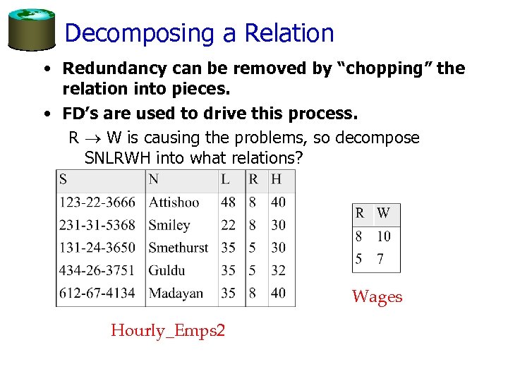Decomposing a Relation • Redundancy can be removed by “chopping” the relation into pieces. • FD’s are used to drive this process. R W is causing the problems, so decompose SNLRWH into what relations? Wages Hourly_Emps 2

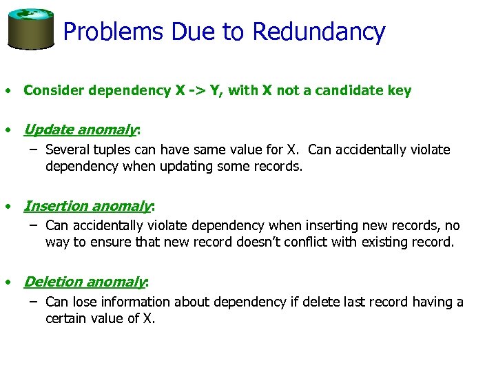Problems Due to Redundancy • Consider dependency X -> Y, with X not a candidate key • Update anomaly: – Several tuples can have same value for X. Can accidentally violate dependency when updating some records. • Insertion anomaly: – Can accidentally violate dependency when inserting new records, no way to ensure that new record doesn’t conflict with existing record. • Deletion anomaly: – Can lose information about dependency if delete last record having a certain value of X.

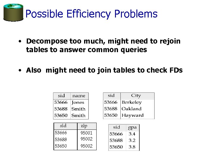Possible Efficiency Problems • Decompose too much, might need to rejoin tables to answer common queries • Also might need to join tables to check FDs sid 53666 53688 53650 zip 95001 95002

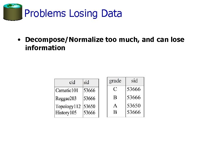Problems Losing Data • Decompose/Normalize too much, and can lose information

Functional Dependencies help us… • …find candidate keys • …know when a table has redundancy • …know when a decomposition is efficient

Where do FDs come from? • They are properties of the real world • When designing database, must find them out based on the characteristics of real world things being modelled. • Database instance can show what FDs do not hold, but can’t really show what FDs are true • Given a set of FDs, can infer other FDs. • F+ = closure of F is the set of all FDs that are implied by F. (includes “trivial dependencies”)

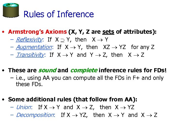Rules of Inference • Armstrong’s Axioms (X, Y, Z are sets of attributes): – Reflexivity: If X Y, then X Y – Augmentation: If X Y, then XZ YZ for any Z – Transitivity: If X Y and Y Z, then X Z • These are sound and complete inference rules for FDs! – i. e. , using AA you can compute all the FDs in F+ and only these FDs. • Some additional rules (that follow from AA): – Union: If X Y and X Z, then X YZ – Decomposition: If X YZ, then X Y and X Z

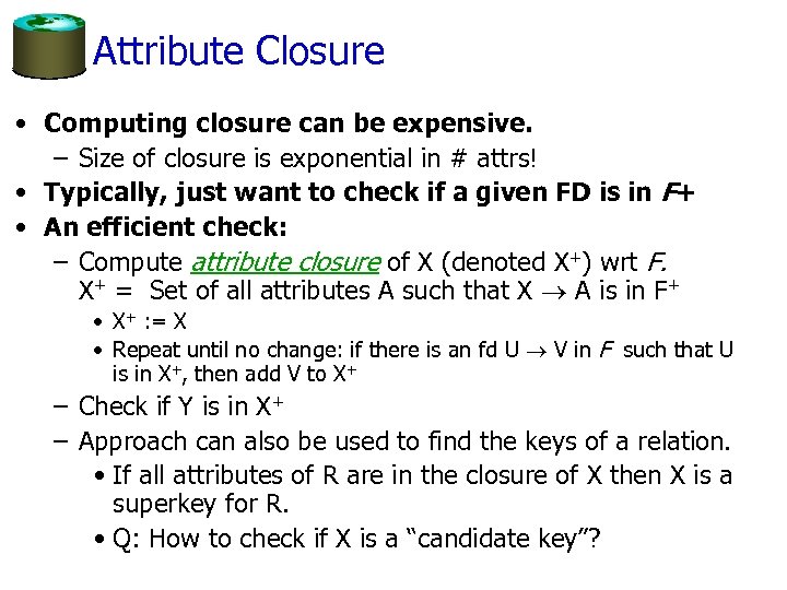Attribute Closure • Computing closure can be expensive. – Size of closure is exponential in # attrs! • Typically, just want to check if a given FD is in F+ • An efficient check: – Compute attribute closure of X (denoted X+) wrt F. X+ = Set of all attributes A such that X A is in F+ • X+ : = X • Repeat until no change: if there is an fd U V in F such that U is in X+, then add V to X+ – Check if Y is in X+ – Approach can also be used to find the keys of a relation. • If all attributes of R are in the closure of X then X is a superkey for R. • Q: How to check if X is a “candidate key”?

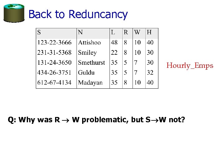Back to Reduncancy Hourly_Emps Q: Why was R W problematic, but S W not?

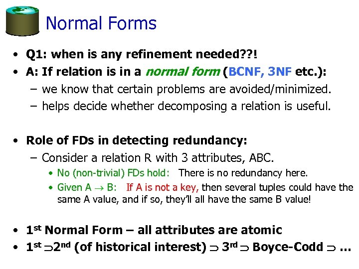Normal Forms • Q 1: when is any refinement needed? ? ! • A: If relation is in a normal form (BCNF, 3 NF etc. ): – we know that certain problems are avoided/minimized. – helps decide whether decomposing a relation is useful. • Role of FDs in detecting redundancy: – Consider a relation R with 3 attributes, ABC. • No (non-trivial) FDs hold: There is no redundancy here. • Given A B: If A is not a key, then several tuples could have the same A value, and if so, they’ll all have the same B value! • 1 st Normal Form – all attributes are atomic • 1 st 2 nd (of historical interest) 3 rd Boyce-Codd …

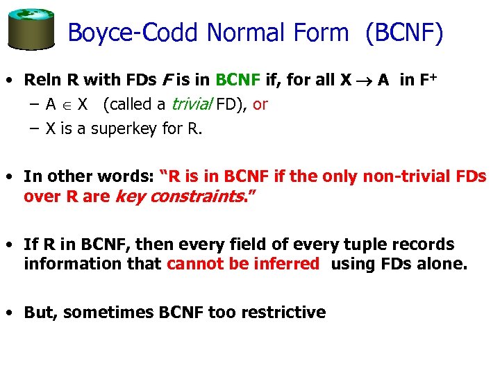Boyce-Codd Normal Form (BCNF) • Reln R with FDs F is in BCNF if, for all X A in F+ – A X (called a trivial FD), or – X is a superkey for R. • In other words: “R is in BCNF if the only non-trivial FDs over R are key constraints. ” • If R in BCNF, then every field of every tuple records information that cannot be inferred using FDs alone. • But, sometimes BCNF too restrictive

Third Normal Form (3 NF) • Reln R with FDs F is in 3 NF if, for all X A in F+ A X (called a trivial FD), or X is a superkey of R, or A is part of some candidate key (not superkey!) for R. (sometimes stated as “A is prime”) • Minimality of a key is crucial in third condition above! • If R is in BCNF, obviously in 3 NF. • If R is in 3 NF, some redundancy is possible. It is a compromise, used when BCNF not achievable (e. g. , no ``good’’ decomp, or performance considerations). – Lossless-join, dependency-preserving decomposition of R into a collection of 3 NF relations always possible.

Decomposition of a Relation Schema • If a relation is not in a desired normal form, it can be decomposed into multiple relations that each are in that normal form. • Suppose that relation R contains attributes A 1. . . An. A decomposition of R consists of replacing R by two or more relations such that: – Each new relation scheme contains a subset of the attributes of R, and – Every attribute of R appears as an attribute of at least one of the new relations.

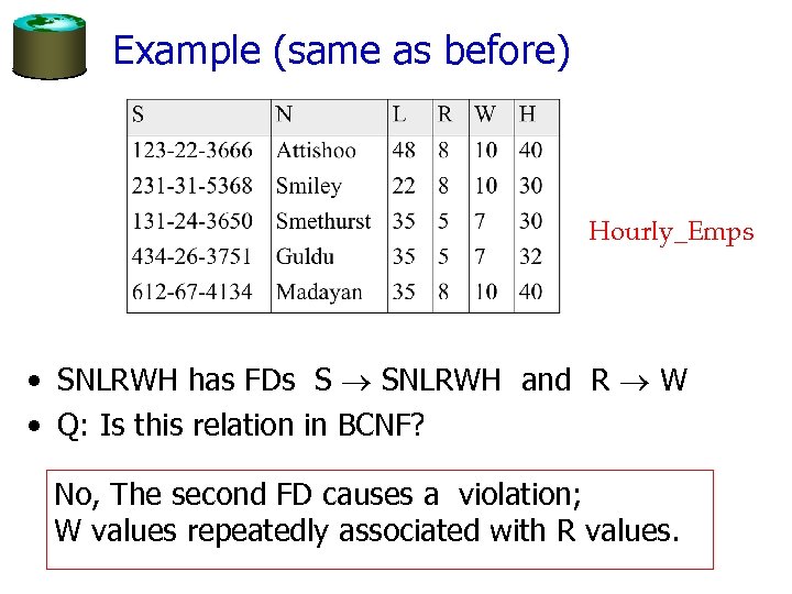Example (same as before) Hourly_Emps • SNLRWH has FDs S SNLRWH and R W • Q: Is this relation in BCNF? No, The second FD causes a violation; W values repeatedly associated with R values.

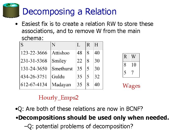Decomposing a Relation • Easiest fix is to create a relation RW to store these associations, and to remove W from the main schema: Wages Hourly_Emps 2 • Q: Are both of these relations are now in BCNF? • Decompositions should be used only when needed. –Q: potential problems of decomposition?

Problems with Decompositions • There are three potential problems to consider: 1) Lossiness: impossible to reconstruct the original relation! • Fortunately, not in the SNLRWH example. 2) Dependency checking may require joins. • Fortunately, not in the SNLRWH example. 3) Some queries become more expensive. • e. g. , How much does Guldu earn? Tradeoff: Must consider these issues vs. redundancy.

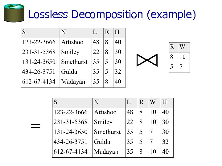Lossless Decomposition (example) =

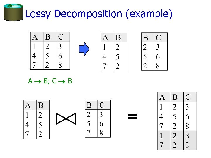Lossy Decomposition (example) A B; C B =

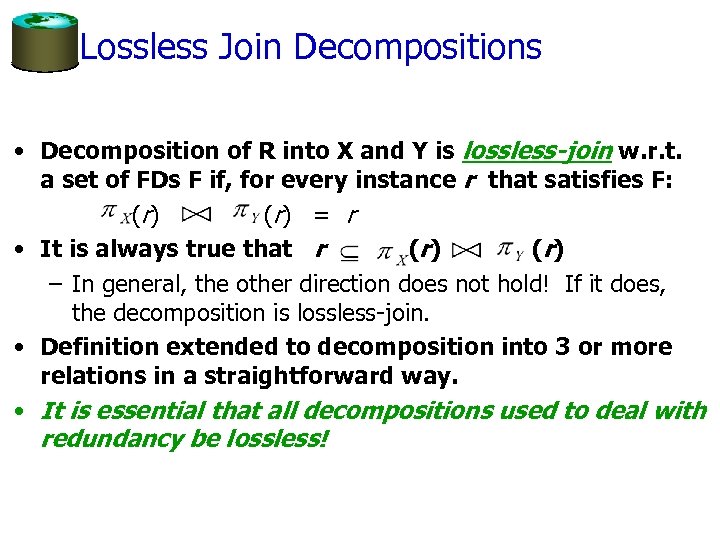Lossless Join Decompositions • Decomposition of R into X and Y is lossless-join w. r. t. a set of FDs F if, for every instance r that satisfies F: ( r) = r • It is always true that r (r ) ( r) – In general, the other direction does not hold! If it does, the decomposition is lossless-join. • Definition extended to decomposition into 3 or more relations in a straightforward way. • It is essential that all decompositions used to deal with redundancy be lossless!

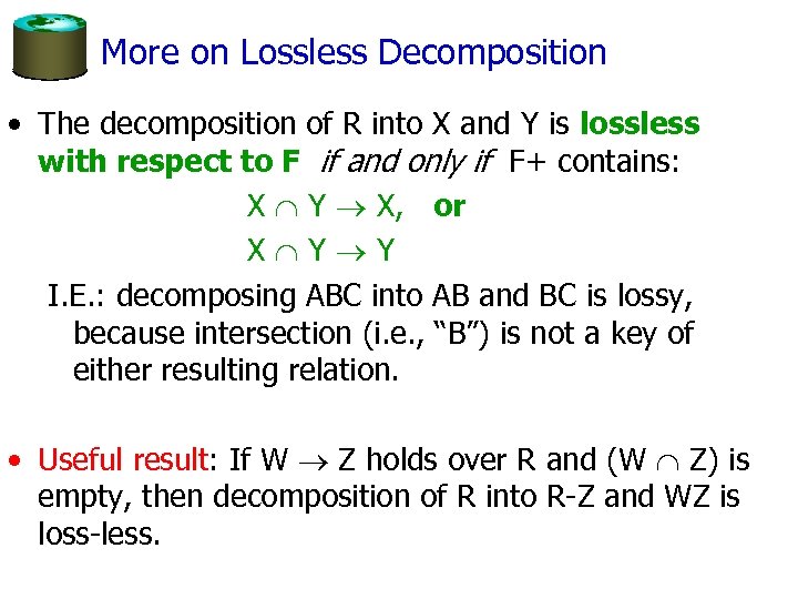More on Lossless Decomposition • The decomposition of R into X and Y is lossless with respect to F if and only if F+ contains: X Y X, or X Y Y I. E. : decomposing ABC into AB and BC is lossy, because intersection (i. e. , “B”) is not a key of either resulting relation. • Useful result: If W Z holds over R and (W Z) is empty, then decomposition of R into R-Z and WZ is loss-less.

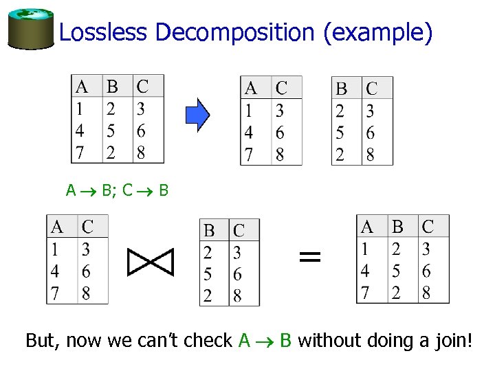Lossless Decomposition (example) A B; C B = But, now we can’t check A B without doing a join!

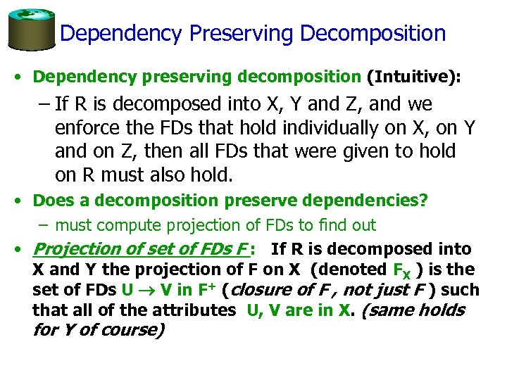Dependency Preserving Decomposition • Dependency preserving decomposition (Intuitive): – If R is decomposed into X, Y and Z, and we enforce the FDs that hold individually on X, on Y and on Z, then all FDs that were given to hold on R must also hold. • Does a decomposition preserve dependencies? – must compute projection of FDs to find out • Projection of set of FDs F : If R is decomposed into X and Y the projection of F on X (denoted FX ) is the set of FDs U V in F+ (closure of F , not just F ) such that all of the attributes U, V are in X. (same holds for Y of course)

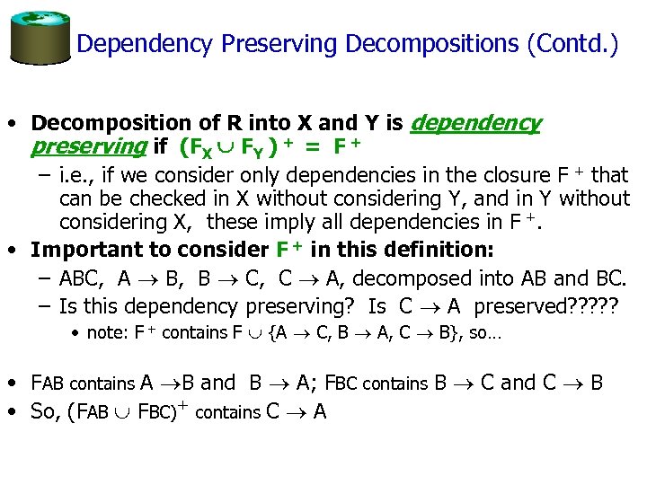Dependency Preserving Decompositions (Contd. ) • Decomposition of R into X and Y is dependency preserving if (FX FY ) + = F + – i. e. , if we consider only dependencies in the closure F + that can be checked in X without considering Y, and in Y without considering X, these imply all dependencies in F +. • Important to consider F + in this definition: – ABC, A B, B C, C A, decomposed into AB and BC. – Is this dependency preserving? Is C A preserved? ? ? • note: F + contains F {A C, B A, C B}, so… • FAB contains A B and B A; FBC contains B C and C B • So, (FAB FBC)+ contains C A

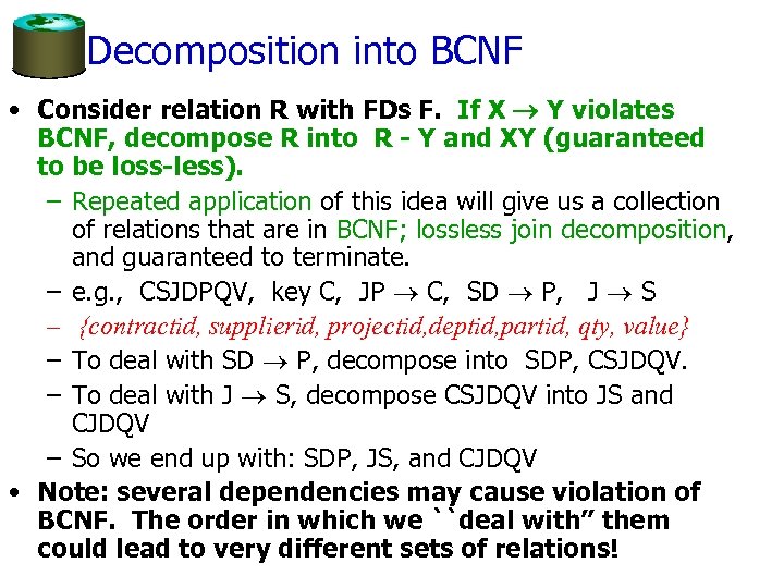Decomposition into BCNF • Consider relation R with FDs F. If X Y violates BCNF, decompose R into R - Y and XY (guaranteed to be loss-less). – Repeated application of this idea will give us a collection of relations that are in BCNF; lossless join decomposition, and guaranteed to terminate. – e. g. , CSJDPQV, key C, JP C, SD P, J S – {contractid, supplierid, projectid, deptid, partid, qty, value} – To deal with SD P, decompose into SDP, CSJDQV. – To deal with J S, decompose CSJDQV into JS and CJDQV – So we end up with: SDP, JS, and CJDQV • Note: several dependencies may cause violation of BCNF. The order in which we ``deal with’’ them could lead to very different sets of relations!

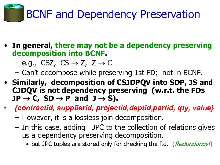BCNF and Dependency Preservation • In general, there may not be a dependency preserving decomposition into BCNF. – e. g. , CSZ, CS Z, Z C – Can’t decompose while preserving 1 st FD; not in BCNF. • Similarly, decomposition of CSJDPQV into SDP, JS and CJDQV is not dependency preserving (w. r. t. the FDs JP C, SD P and J S). • {contractid, supplierid, projectid, deptid, partid, qty, value} – However, it is a lossless join decomposition. – In this case, adding JPC to the collection of relations gives us a dependency preserving decomposition. • but JPC tuples are stored only for checking the f. d. (Redundancy!)

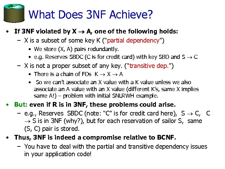What Does 3 NF Achieve? • If 3 NF violated by X A, one of the following holds: – X is a subset of some key K (“partial dependency”) • We store (X, A) pairs redundantly. • e. g. Reserves SBDC (C is for credit card) with key SBD and S C – X is not a proper subset of any key. (“transitive dep. ”) • There is a chain of FDs K X A • So we can’t associate an X value with a K value unless we also associate an A value with an X value (different K’s, same X implies same A!) – problem with initial SNLRWH example. • But: even if R is in 3 NF, these problems could arise. – e. g. , Reserves SBDC (note: “C” is for credit card here), S C, C S is in 3 NF (why? ), but for each reservation of sailor S, same (S, C) pair is stored. • Thus, 3 NF is indeed a compromise relative to BCNF. – You have to deal with the partial and transitive dependency issues in your application code!

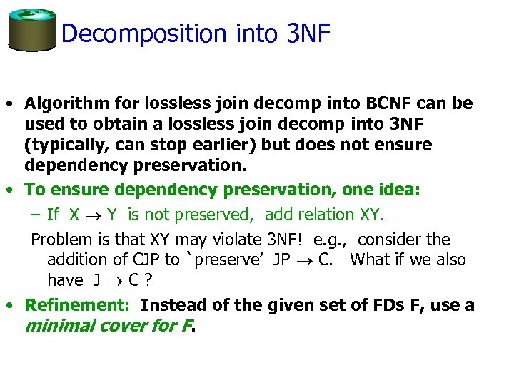Decomposition into 3 NF • Algorithm for lossless join decomp into BCNF can be used to obtain a lossless join decomp into 3 NF (typically, can stop earlier) but does not ensure dependency preservation. • To ensure dependency preservation, one idea: – If X Y is not preserved, add relation XY. Problem is that XY may violate 3 NF! e. g. , consider the addition of CJP to `preserve’ JP C. What if we also have J C ? • Refinement: Instead of the given set of FDs F, use a minimal cover for F.

Minimal Cover for a Set of FDs • Minimal cover G for a set of FDs F: – Closure of F = closure of G. – Right hand side of each FD in G is a single attribute. – If we modify G by deleting an FD or by deleting attributes from an FD in G, the closure changes. • Intuitively, every FD in G is needed, and ``as small as possible’’ in order to get the same closure as F. • e. g. , A B, ABCD E, EF GH, ACDF EG has the following minimal cover: – A B, ACD E, EF G and EF H • M. C. implies Lossless-Join, Dep. Pres. Decomp!!! – (in book)

Summary of Schema Refinement • BCNF: each field contains information that cannot be inferred using only FDs. – ensuring BCNF is a good heuristic. • Not in BCNF? Try decomposing into BCNF relations. – Must consider whether all FDs are preserved! • Lossless-join, dependency preserving decomposition into BCNF impossible? Consider 3 NF. – Same if BCNF decomp is unsuitable for typical queries – Decompositions should be carried out and/or re-examined while keeping performance requirements in mind. • Note: even more restrictive Normal Forms exist (we don’t cover them in this course, but some are in the book. )