Foundations of Software Testing Chapter 3 Test Generation

Foundations of Software Testing Chapter 3: Test Generation: Finite State Models Aditya P. Mathur Purdue University These slides are copyrighted. They are for use with the Foundations of Software Testing book by Aditya Mathur. Please use the slides but do not remove the copyright notice. Last update: September 3, 2007

Learning Objectives § What are Finite State Models? § The W method for test generation § The Wp method for test generation © Aditya P. Mathur 2007 2

Where are FSMs used? § Conformance testing of communications protocols--this is where it all started. § Testing of any system/subsystem modeled as a finite state machine, e. g. elevator designs, automobile components (locks, transmission, stepper motors, etc), nuclear plant protection systems, steam boiler control, etc. ) § Finite state machines are widely used in modeling of all kinds of systems. Generation of tests from FSM specifications assists in testing the conformance of implementations to the corresponding FSM model. © Aditya P. Mathur 2007 3

Where are FSMs used? Modeling GUIs, network protocols, pacemakers, Teller machines, WEB applications, safety software modeling in nuclear plants, and many more. While the FSM’s considered in examples are abstract machines, they are abstractions of many real-life machines. © Aditya P. Mathur 2007 4

What is an Finite State Machine? Quick review • A finite state machine, abbreviated as FSM, is an abstract representation of behavior exhibited by some systems. • An FSM is derived from application requirements. For example, a network protocol could be modeled using an FSM. • Not all aspects of an application’s requirements are specified by an FSM. Real time requirements, performance requirements, and several types of computational requirements cannot be specified by an FSM. © Aditya P. Mathur 2007 5

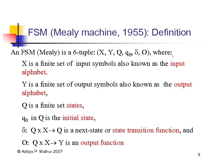FSM (Mealy machine, 1955): Definition An FSM (Mealy) is a 6 -tuple: (X, Y, Q, q 0, , O), where: , X is a finite set of input symbols also known as the input alphabet. Y is a finite set of output symbols also known as the output alphabet, Q is a finite set states, q 0 in Q is the initial state, : Q x X Q is a next-state or state transition function, and O: Q x X Y is an output function © Aditya P. Mathur 2007 6

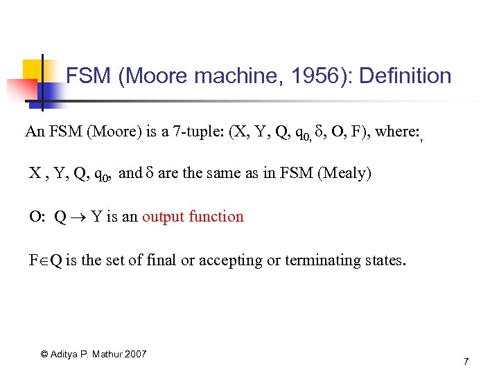FSM (Moore machine, 1956): Definition An FSM (Moore) is a 7 -tuple: (X, Y, Q, q 0, , O, F), where: , X , Y, Q, q 0, and are the same as in FSM (Mealy) O: Q Y is an output function F Q is the set of final or accepting or terminating states. © Aditya P. Mathur 2007 7

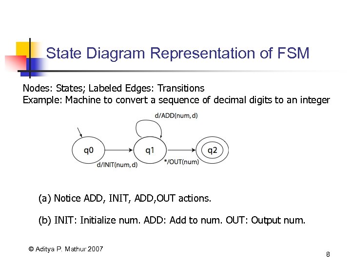State Diagram Representation of FSM Nodes: States; Labeled Edges: Transitions Example: Machine to convert a sequence of decimal digits to an integer (a) Notice ADD, INIT, ADD, OUT actions. (b) INIT: Initialize num. ADD: Add to num. OUT: Output num. © Aditya P. Mathur 2007 8

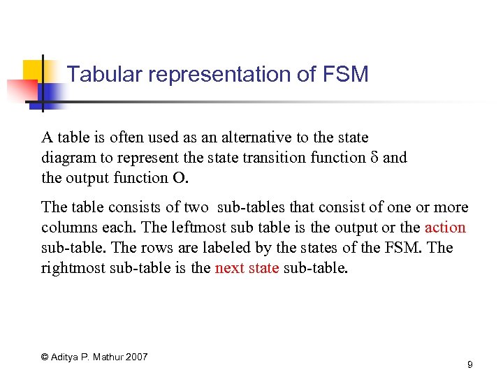Tabular representation of FSM A table is often used as an alternative to the state diagram to represent the state transition function and the output function O. The table consists of two sub-tables that consist of one or more columns each. The leftmost sub table is the output or the action sub-table. The rows are labeled by the states of the FSM. The rightmost sub-table is the next state sub-table. © Aditya P. Mathur 2007 9

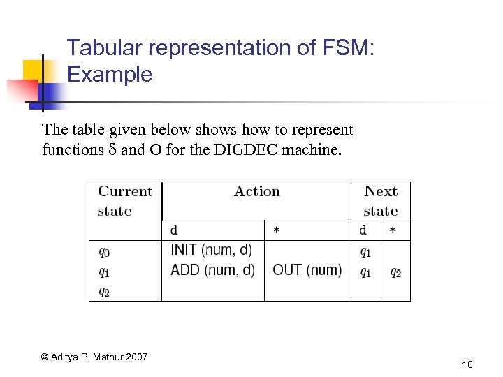Tabular representation of FSM: Example The table given below shows how to represent functions and O for the DIGDEC machine. © Aditya P. Mathur 2007 10

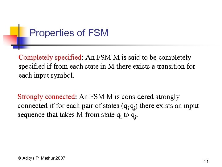Properties of FSM Completely specified: An FSM M is said to be completely specified if from each state in M there exists a transition for each input symbol. Strongly connected: An FSM M is considered strongly connected if for each pair of states (qi qj) there exists an input sequence that takes M from state qi to qj. © Aditya P. Mathur 2007 11

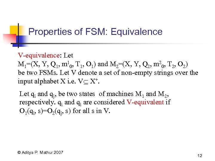Properties of FSM: Equivalence V-equivalence: Let M 1=(X, Y, Q 1, m 10, T 1, O 1) and M 2=(X, Y, Q 2, m 20, T 2, O 2) be two FSMs. Let V denote a set of non-empty strings over the input alphabet X i. e. V X+. Let qi and qj, be two states of machines M 1 and M 2, respectively. qi and qi are considered V-equivalent if O 1(qi, s)=O 2(qj, s) for all s in V. © Aditya P. Mathur 2007 12

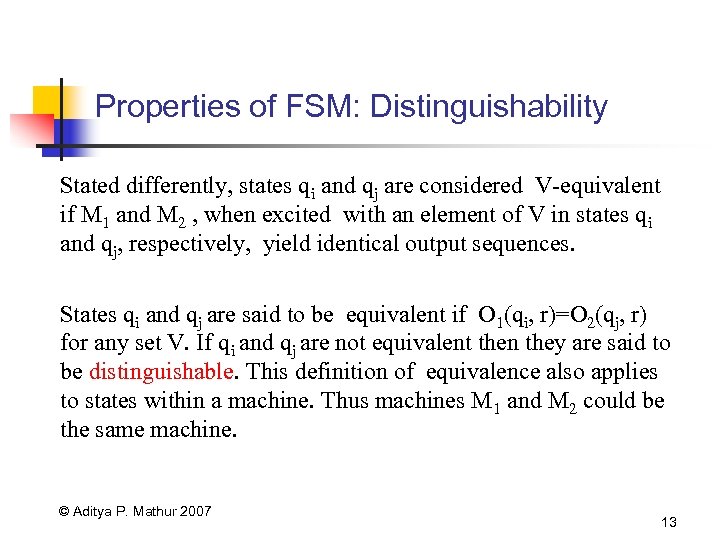Properties of FSM: Distinguishability Stated differently, states qi and qj are considered V-equivalent if M 1 and M 2 , when excited with an element of V in states qi and qj, respectively, yield identical output sequences. States qi and qj are said to be equivalent if O 1(qi, r)=O 2(qj, r) for any set V. If qi and qj are not equivalent then they are said to be distinguishable. This definition of equivalence also applies to states within a machine. Thus machines M 1 and M 2 could be the same machine. © Aditya P. Mathur 2007 13

Properties of FSM: k-equivalence: Let M 1=(X, Y, Q 1, m 10, T 1, O 1) and M 2=(X, Y, Q 2, m 20, T 2, O 2) be two FSMs. States qi Q 1 and qj Q 2 are considered k-equivalent if, when excited by any input of length k, yield identical output sequences. © Aditya P. Mathur 2007 14

Properties of FSM: k-equivalence (contd. ) States that are not k-equivalent are considered k-distinguishable. Once again, M 1 and M 2 may be the same machines implying that k-distinguishability applies to any pair of states of an FSM. It is also easy to see that if two states are k-distinguishable for any k>0 then they are also distinguishable for any n k. If M 1 and M 2 are not k-distinguishable then they are said to be kequivalent. © Aditya P. Mathur 2007 15

Properties of FSM: Machine Equivalence Machine equivalence: Machines M 1 and M 2 are said to be equivalent if (a) for each state in M 1 there exists a state ' in M 2 such that and ' are equivalent and (b) for each state in M 2 there exists a state ' in M 1 such that and ' are equivalent. Machines that are not equivalent are considered distinguishable. Minimal machine: An FSM M is considered minimal if the number of states in M is less than or equal to any other FSM equivalent to M. © Aditya P. Mathur 2007 16

Faults Targeted © Aditya P. Mathur 2007 17

Faults in implementation An FSM serves to specify the correct requirement or design of an application. Hence tests generated from an FSM target faults related to the FSM itself. What faults are targeted by the tests generated using an FSM? © Aditya P. Mathur 2007 18

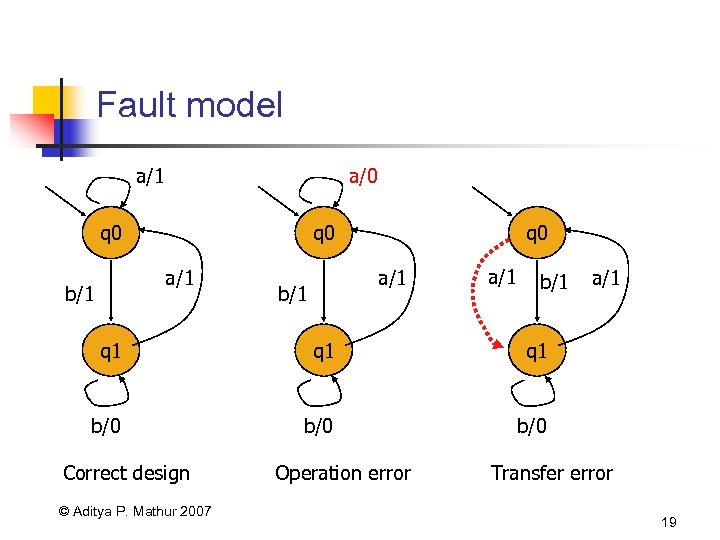Fault model a/1 a/0 q 0 a/1 b/1 q 1 q 1 b/0 a/1 b/0 Correct design © Aditya P. Mathur 2007 Operation error Transfer error 19

Fault model (contd. ) a/1 b/1 a/0 q 0 a/1 q 2 a/1 b/0 q 1 b/0 Extra state error © Aditya P. Mathur 2007 Missing state error 20

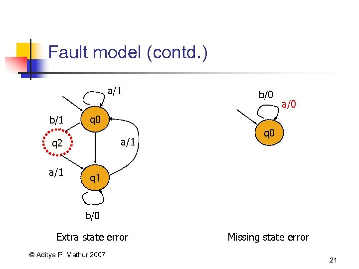Fault model (contd. ) a/1 b/1 a/0 q 0 a/1 q 2 a/1 b/0 q 1 b/0 Extra state error © Aditya P. Mathur 2007 Missing state error 21

Test generation using Chow’s method © Aditya P. Mathur 2007 22

Assumptions for test generation 1. M is Completely specified, minimal, connected, and deterministic. 2. M starts in a fixed initial state. 3. M and IUT (Implementation Under Test) have the same input alphabet. © Aditya P. Mathur 2007 23

Overall algorithm used in Chow’s method Step 1: Estimate the maximum number of states (m) in the correct implementation of the given FSM M. Step 2: Construct the characterization set W for M. Step 3: (a) Construct the testing tree for M and (b) generate the transition cover set P from the testing tree. Step 4: Construct set Z from W and m. Step 5: Desired test set=P. Z © Aditya P. Mathur 2007 24

Step 1: Estimation of m This is based on a knowledge of the implementation. In the absence of any such knowledge, let m=number of states in M. © Aditya P. Mathur 2007 25

Step 2: Construction of W. What is W? Let M=(X, Y, Q, q 1, , O) be a minimal and complete FSM. W is a finite set of input sequences that distinguish the behavior of any pair of states in M. Each input sequence in W is of finite length. Given states qi and qj in Q, W contains a string s such that: O(qi, s) O(qj, s) © Aditya P. Mathur 2007 26

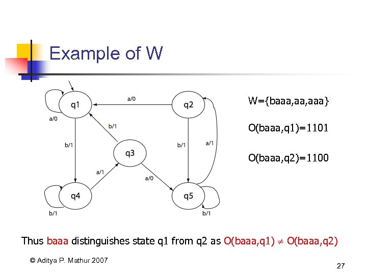Example of W W={baaa, aaa} O(baaa, q 1)=1101 O(baaa, q 2)=1100 Thus baaa distinguishes state q 1 from q 2 as O(baaa, q 1) O(baaa, q 2) © Aditya P. Mathur 2007 27

Steps in the construction of W Step 1: Construct a sequence of k-equivalence partitions of Q denoted as P 1, P 2, …Pm, m>0. Step 2: Traverse the k-equivalence partitions in reverse order to obtain distinguishing sequence for each pair of states. © Aditya P. Mathur 2007 28

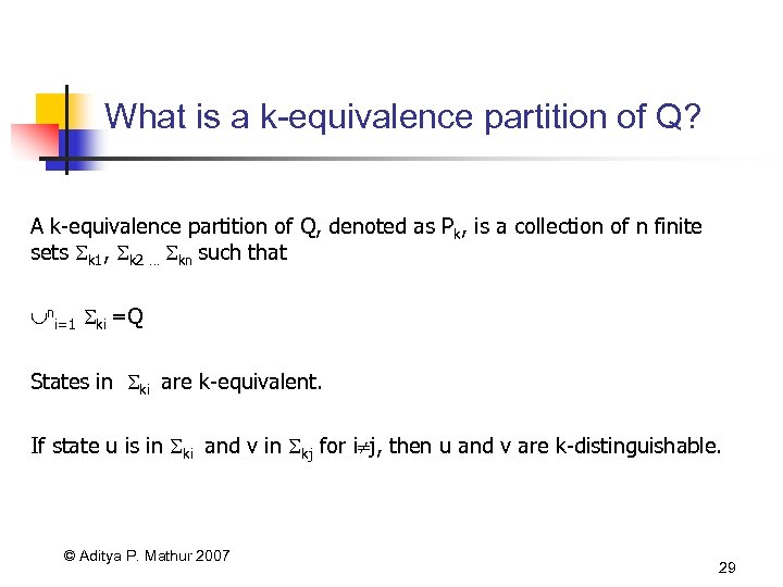What is a k-equivalence partition of Q? A k-equivalence partition of Q, denoted as Pk, is a collection of n finite sets k 1, k 2 … kn such that ni=1 ki =Q States in ki are k-equivalent. If state u is in ki and v in kj for i j, then u and v are k-distinguishable. © Aditya P. Mathur 2007 29

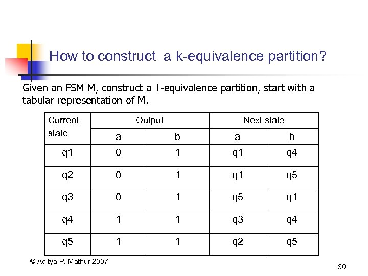How to construct a k-equivalence partition? Given an FSM M, construct a 1 -equivalence partition, start with a tabular representation of M. Current state Output Next state a b q 1 0 1 q 4 q 2 0 1 q 5 q 3 0 1 q 5 q 1 q 4 1 1 q 3 q 4 q 5 1 1 q 2 q 5 © Aditya P. Mathur 2007 30

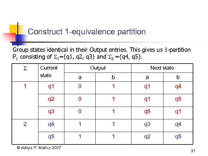Construct 1 -equivalence partition Group states identical in their Output entries. This gives us 1 -partition P 1 consisting of 1={q 1, q 2, q 3} and 2 ={q 4, q 5}. Current state Output Next state a b q 1 0 1 q 4 0 1 q 5 q 3 0 1 q 5 q 1 q 4 1 1 q 3 q 4 q 5 2 b q 2 1 a 1 1 q 2 q 5 © Aditya P. Mathur 2007 31

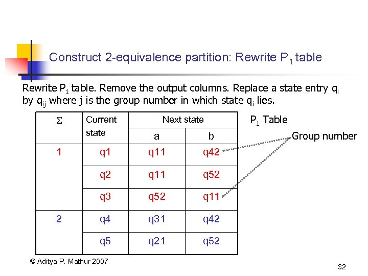Construct 2 -equivalence partition: Rewrite P 1 table. Remove the output columns. Replace a state entry q i by qij where j is the group number in which state qi lies. Current state P 1 Table Next state q 11 q 52 q 11 q 4 q 31 q 42 q 5 q 21 Group number q 42 q 3 2 b q 2 1 a q 52 © Aditya P. Mathur 2007 32

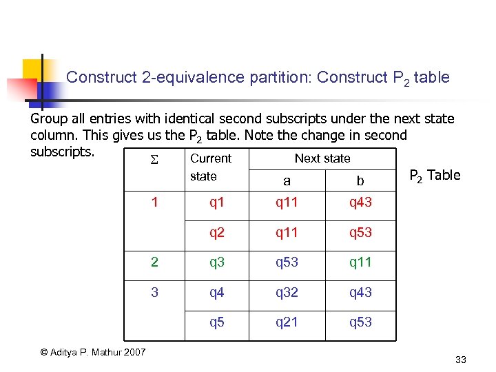Construct 2 -equivalence partition: Construct P 2 table Group all entries with identical second subscripts under the next state column. This gives us the P 2 table. Note the change in second subscripts. Current Next state P 2 Table state a b 1 q 11 q 43 q 2 q 11 q 53 2 q 3 q 53 q 11 3 q 4 q 32 q 43 q 5 © Aditya P. Mathur 2007 q 1 q 21 q 53 33

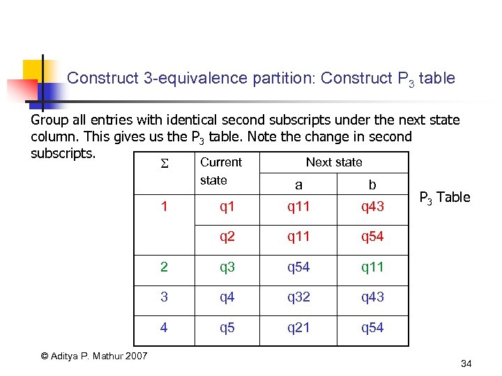Construct 3 -equivalence partition: Construct P 3 table Group all entries with identical second subscripts under the next state column. This gives us the P 3 table. Note the change in second subscripts. Current Next state a b q 11 q 43 q 2 q 11 q 54 2 q 3 q 54 q 11 3 q 4 q 32 q 43 4 q 5 q 21 q 54 1 © Aditya P. Mathur 2007 P 3 Table 34

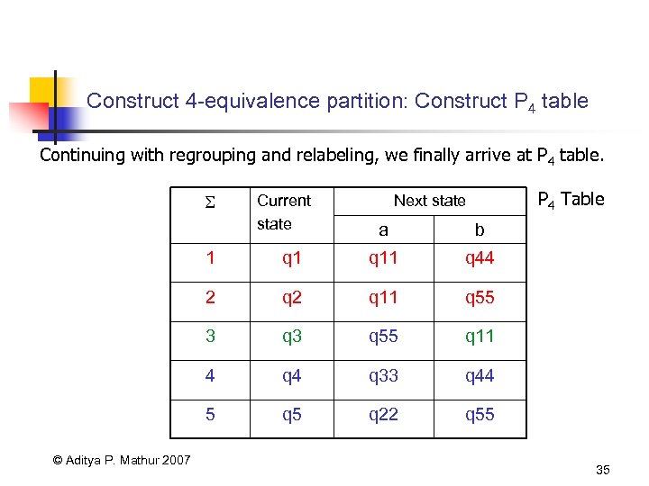Construct 4 -equivalence partition: Construct P 4 table Continuing with regrouping and relabeling, we finally arrive at P 4 table. Current state P 4 Table Next state a b 1 q 11 q 44 2 q 11 q 55 3 q 55 q 11 4 q 33 q 44 5 © Aditya P. Mathur 2007 q 1 q 5 q 22 q 55 35

k-equivalence partition: Convergence The process is guaranteed to converge. When the process converges, and the machine is minimal, each state will be in a separate group. The next step is to obtain the distinguishing strings for each state. © Aditya P. Mathur 2007 36

Finding the distinguishing sequences: Example Let us find a distinguishing sequence for states q 1 and q 2. Find tables Pi and Pi+1 such that (q 1, q 2) are in the same group in Pi and different groups in Pi+1. We get P 3 and P 4. Initialize z=. Find the input symbol that distinguishes q 1 and q 2 in table P 3. This symbol is b. We update z to z. b. Hence z now becomes b. © Aditya P. Mathur 2007 37

Finding the distinguishing sequences: Example (contd. ) The next states for q 1 and q 2 on b are, respectively, q 4 and q 5. We move to the P 2 table and find the input symbol that distinguishes q 4 and q 5. Let us select a as the distinguishing symbol. Update which now becomes ba. The next states for states q 4 and q 5 on symbol a are, respectively, q 3 and q 2. These two states are distinguished in P 1 by a and b. Let us select a. We update z to baa. © Aditya P. Mathur 2007 38

Finding the distinguishing sequences: Example (contd. ) The next states for q 3 and q 2 on a are, respectively, q 1 and q 5. Moving to the original state transition table we obtain a as the distinguishing symbol for q 1 and q 5 We update z to baaa. This is the farthest we can go backwards through the various tables. baaa is the desired distinguishing sequence for states q 1 and q 2. Check that o(q 1, baaa) o(q 2, baaa). © Aditya P. Mathur 2007 39

Finding the distinguishing sequences: Example (contd. ) Using the same procedure used for q 1 and q 2, we can find the distinguishing sequence for each pair of states. This leads us to the following characterization set for our FSM. W={a, aaa, baaa} © Aditya P. Mathur 2007 40

Chow’s method: where are we? Step 1: Estimate the maximum number of states (m) in the correct implementation of the given FSM M. Done Step 2: Construct the characterization set W for M. Step 3: (a) Construct the testing tree for M and (b) generate the Next (a) transition cover set P from the testing tree. Step 4: Construct set Z from W and m. Step 5: Desired test set=P. Z © Aditya P. Mathur 2007 41

Step 3: (a) Construct the testing tree for M A testing tree of an FSM is a tree rooted at the initial state. It contains at least one path from the initial state to the remaining states in the FSM. Here is how we construct the testing tree. State q 0, the initial state, is the root of the testing tree. Suppose that the testing tree has been constructed until level k. The (k+1)th level is built as follows. Select a node n at level k. If n appears at any level from 1 through k-1 , then n is a leaf node and is not expanded any further. If n is not a leaf node then we expand it by adding a branch from node n to a new node m if (n, x)=m for each x in X. This branch is labeled as x. This step is repeated for all nodes at level k. © Aditya P. Mathur 2007 42

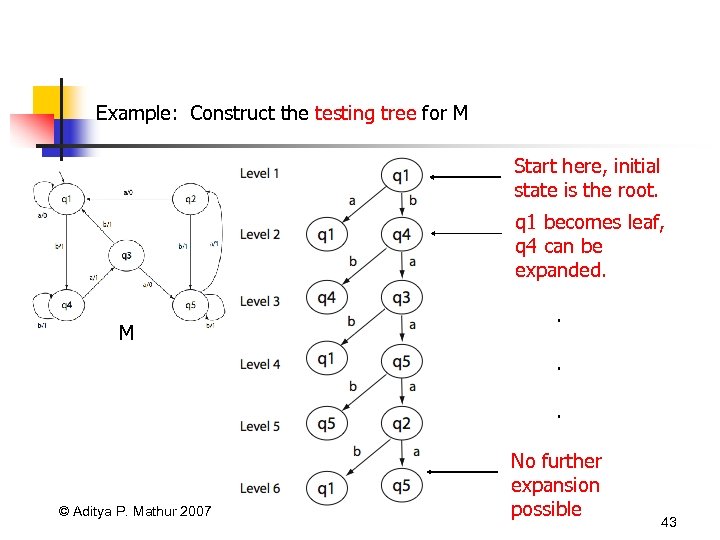Example: Construct the testing tree for M Start here, initial state is the root. q 1 becomes leaf, q 4 can be expanded. M . . . © Aditya P. Mathur 2007 No further expansion possible 43

Chow’s method: where are we? Step 1: Estimate the maximum number of states (m) in the correct implementation of the given FSM M. Done Step 2: Construct the characterization set W for M. Step 3: (a) Construct the testing tree for M and (b) generate the Next, (b) transition cover set P from the testing tree. Step 4: Construct set Z from W and m. Step 5: Desired test set=P. Z © Aditya P. Mathur 2007 44

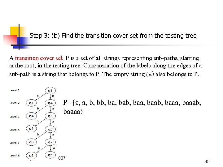Step 3: (b) Find the transition cover set from the testing tree A transition cover set P is a set of all strings representing sub-paths, starting at the root, in the testing tree. Concatenation of the labels along the edges of a sub-path is a string that belongs to P. The empty string ( ) also belongs to P. P={ , a, b, ba, bab, baab, baaab, baaaa} © Aditya P. Mathur 2007 45

Chow’s method: where are we? Step 1: Estimate the maximum number of states (m) in the correct implementation of the given FSM M. Done Step 2: Construct the characterization set W for M. Step 3: (a) Construct the testing tree for M and (b) generate the Done transition cover set P from the testing tree. Step 4: Construct set Z from W and m. Next Step 5: Desired test set=P. Z © Aditya P. Mathur 2007 46

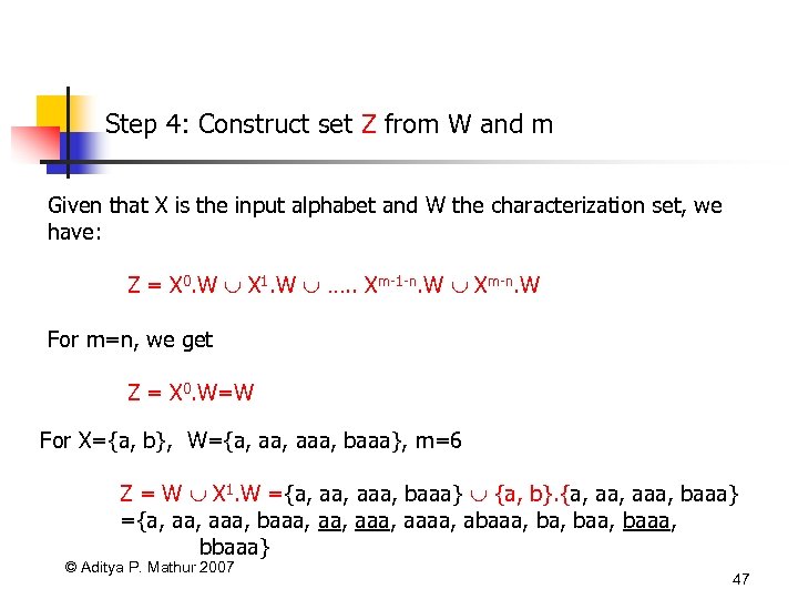Step 4: Construct set Z from W and m Given that X is the input alphabet and W the characterization set, we have: Z = X 0. W X 1. W …. . Xm-1 -n. W Xm-n. W For m=n, we get Z = X 0. W=W For X={a, b}, W={a, aaa, baaa}, m=6 Z = W X 1. W ={a, aaa, baaa} {a, b}. {a, aaa, baaa} ={a, aaa, baaa, abaaa, baa, baaa, bbaaa} © Aditya P. Mathur 2007 47

Chow’s method: where are we? Step 1: Estimate the maximum number of states (m) in the correct implementation of the given FSM M. Done Step 2: Construct the characterization set W for M. Step 3: (a) Construct the testing tree for M and (b) generate the Done transition cover set P from the testing tree. Step 4: Construct set Z from W and m. Step 5: Desired test set=P. Z © Aditya P. Mathur 2007 Done Next 48

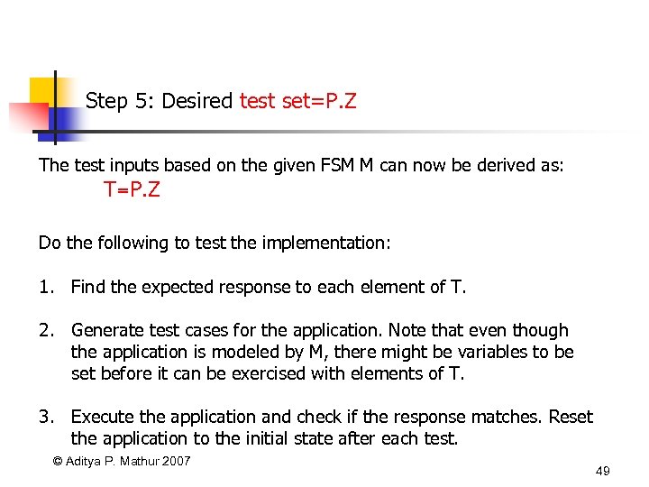Step 5: Desired test set=P. Z The test inputs based on the given FSM M can now be derived as: T=P. Z Do the following to test the implementation: 1. Find the expected response to each element of T. 2. Generate test cases for the application. Note that even though the application is modeled by M, there might be variables to be set before it can be exercised with elements of T. 3. Execute the application and check if the response matches. Reset the application to the initial state after each test. © Aditya P. Mathur 2007 49

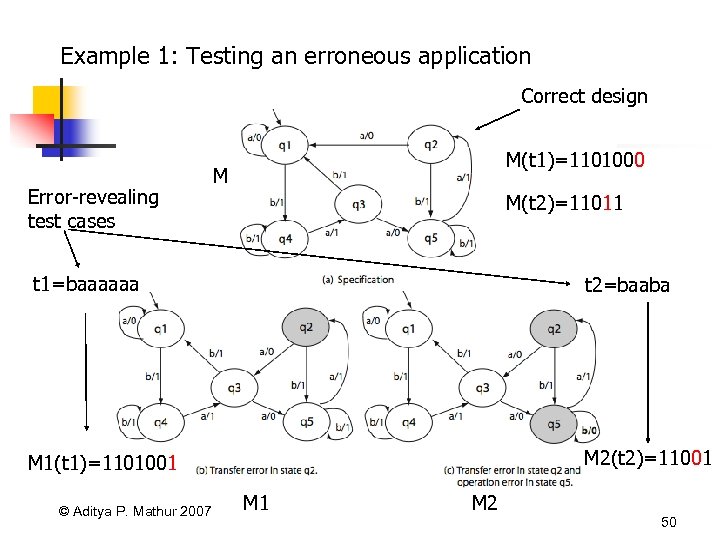Example 1: Testing an erroneous application Correct design Error-revealing test cases M(t 1)=1101000 M M(t 2)=11011 t 1=baaaaaa t 2=baaba M 1(t 1)=1101001 M 2(t 2)=11001 © Aditya P. Mathur 2007 M 1 M 2 50

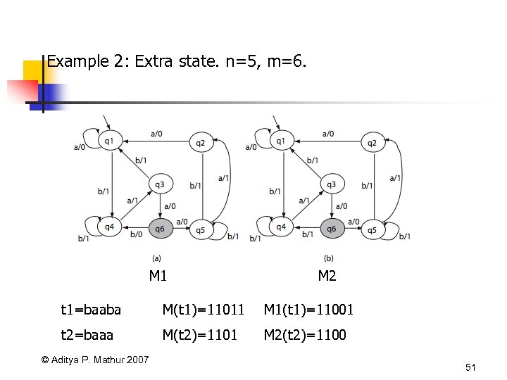Example 2: Extra state. n=5, m=6. M 1 M 2 t 1=baaba M(t 1)=11011 M 1(t 1)=11001 t 2=baaa M(t 2)=1101 M 2(t 2)=1100 © Aditya P. Mathur 2007 51

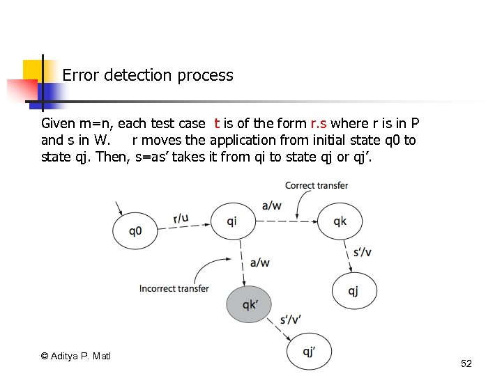Error detection process Given m=n, each test case t is of the form r. s where r is in P and s in W. r moves the application from initial state q 0 to state qj. Then, s=as’ takes it from qi to state qj or qj’. © Aditya P. Mathur 2007 52

The Partial W (Wp) method © Aditya P. Mathur 2007 53

The partial W (Wp) method Tests are generated from minimal, complete, and connected FSM. Size of tests generated is generally smaller than that generated using the W-method. Test generation process is divided into two phases: Phase 1: Generate a test set using the state cover set (S) and the characterization set (W). Phase 2: Generate additional tests using a subset of the transition cover set and state identification sets. What is a state cover set? A state identification set? © Aditya P. Mathur 2007 54

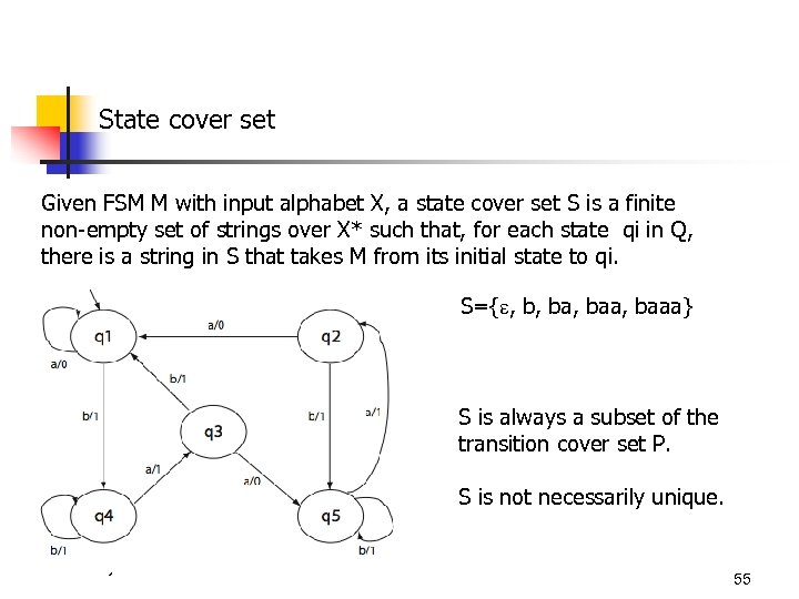State cover set Given FSM M with input alphabet X, a state cover set S is a finite non-empty set of strings over X* such that, for each state qi in Q, there is a string in S that takes M from its initial state to qi. S={ , b, baa, baaa} S is always a subset of the transition cover set P. S is not necessarily unique. © Aditya P. Mathur 2007 55

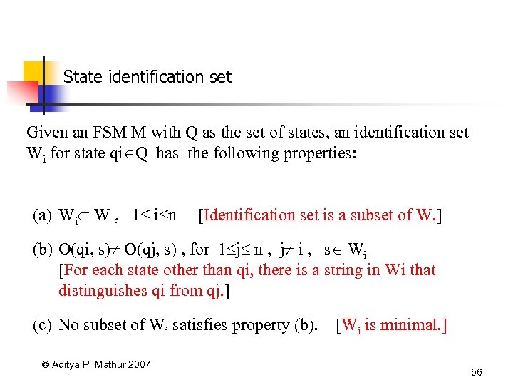State identification set Given an FSM M with Q as the set of states, an identification set Wi for state qi Q has the following properties: (a) Wi W , 1 i n [Identification set is a subset of W. ] (b) O(qi, s) O(qj, s) , for 1 j n , j i , s Wi [For each state other than qi, there is a string in Wi that distinguishes qi from qj. ] (c) No subset of Wi satisfies property (b). © Aditya P. Mathur 2007 [Wi is minimal. ] 56

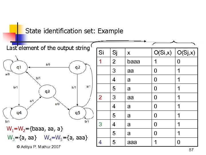State identification set: Example Last element of the output string Si Sj x O(Si, x) O(Sj, x) 1 2 baaa 1 0 3 aa 0 1 4 a 0 1 5 aaa 1 0 2 W 1=W 2={baaa, a} W 3={a, aa} W 4=W 5={a, aaa} © Aditya P. Mathur 2007 3 4 57

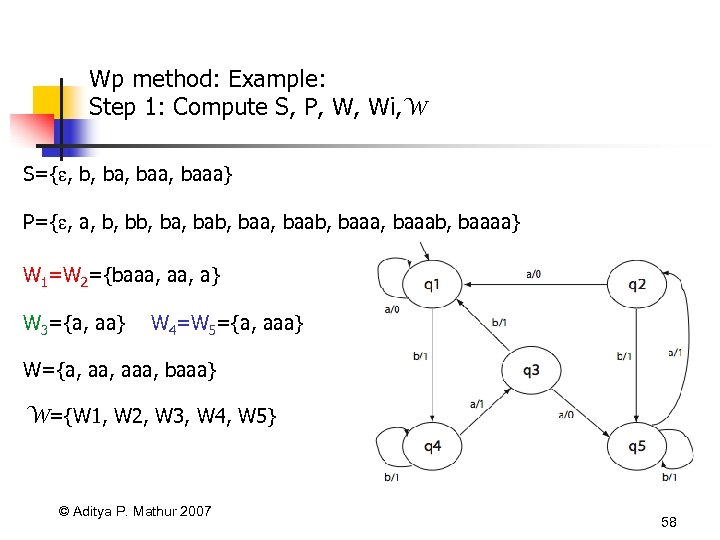Wp method: Example: Step 1: Compute S, P, W, Wi, W S={ , b, baa, baaa} P={ , a, b, ba, bab, baab, baaab, baaaa} W 1=W 2={baaa, a} W 3={a, aa} W 4=W 5={a, aaa} W={a, aaa, baaa} W={W 1, W 2, W 3, W 4, W 5} © Aditya P. Mathur 2007 58

Wp method: Example: Step 2: Compute T 1 [m=n] T 1 = S. W = { , b, baa, baaa}. {a, aaa, baaa} Elements of T 1 ensure that the each state of the FSM is covered and distinguished from the remaining states. © Aditya P. Mathur 2007 59

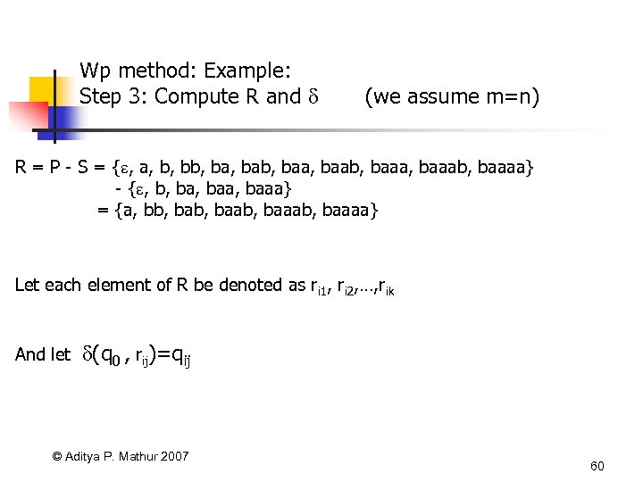Wp method: Example: Step 3: Compute R and (we assume m=n) R = P - S = { , a, b, ba, bab, baab, baaab, baaaa} - { , b, baa, baaa} = {a, bb, baab, baaaa} Let each element of R be denoted as ri 1, ri 2, …, rik And let (q 0 , rij)=qij © Aditya P. Mathur 2007 60

Wp method: Example: Step 4: Compute T 2 [m=n] T 2=R W= kj=1 ({rij}. Wij ), where Wij is the identification set for state qij. (q 1, a)=q 1 (q 1, bb)=q 4 (q 1, bab)=q 1 (q 1, baab)=q 5 (q 1, baaaa)=q 1 T 2 = ({a}. W 1 ) ({bb}. W 4 ) ({bab}. W 1 ) ({baab}. W 5 ) ({baaaa}. W 1 ) = {abaaa, aa} {bba, bbaaa} {babbaaa, baba} {baaba, baabaaa} {baaaba, baaa} {baaaabaaa, baaaaa} © Aditya P. Mathur 2007 61

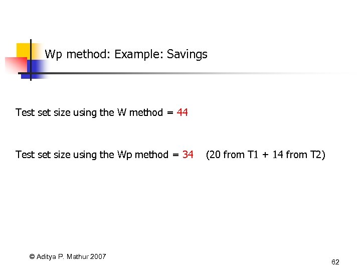Wp method: Example: Savings Test set size using the W method = 44 Test set size using the Wp method = 34 © Aditya P. Mathur 2007 (20 from T 1 + 14 from T 2) 62

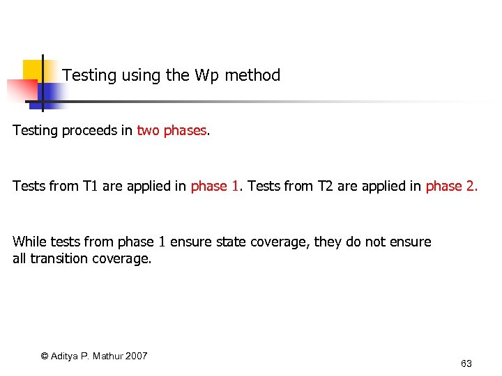Testing using the Wp method Testing proceeds in two phases. Tests from T 1 are applied in phase 1. Tests from T 2 are applied in phase 2. While tests from phase 1 ensure state coverage, they do not ensure all transition coverage. © Aditya P. Mathur 2007 63

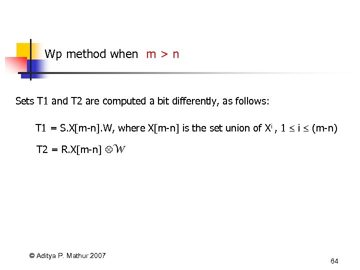Wp method when m > n Sets T 1 and T 2 are computed a bit differently, as follows: T 1 = S. X[m-n]. W, where X[m-n] is the set union of Xi , 1 i (m-n) T 2 = R. X[m-n] W © Aditya P. Mathur 2007 64

Summary Behavior of a large variety of applications can be modeled using finite state machines (FSM). GUIs can also be modeled using FSMs The W and the Wp methods are automata theoretic methods to generate tests from a given FSM model. Tests so generated are guaranteed to detect all operation errors, transfer errors, and missing/extra state errors in the implementation given that the FSM representing the implementation is complete, connected, and minimal. What happens if it is not? The size of tests sets generated by the W method is larger than that generated by the Wp method while their fault detection effectiveness are the same. © Aditya P. Mathur 2007 65