93b4f5a0859d5f3730c29d2142f6d8b9.ppt
- Количество слайдов: 57


Forest Disturbance Mapping @ USFS RSAC September 6, 2007 USDA Forest Service, Remote Sensing Application Center, http: //fsweb. rsac. fs. fed. us/

Remote Sensing Applications Center • Provide remote sensing and analysis expertise to clients in all parts of USFS – – NFS (National, Regional, Forest, District) Research (e. g. , FIA) State & Private (e. g. , FHM/FHP) Centers and Enterprise Teams (e. g. , FHTET) • Other cooperators include National Park Service, BLM, NASA, etc. • Currently working with FHTET to produce an operational, near real-time, forest disturbance detection system that is scalable to national level

Prior & Concurrent Broad-scale Forest Change Detection Work U. S. -wide forest disturbance maps (FHTET) MODIS continuous disturbance estimation studies (FIA) Rapid forest damage mapping in response to sudden major events (FIA) Southern pine beetle infestation mapping - cooperative project with NFS Southern region - compare MODIS and AWi. FS

National disturbance maps • First project estimated forest disturbance in western U. S. , 2000 -05 • 8 -day composites, fused 250 m and 500 m. Simple difference based on anniversary images. • Empirical ecosystem-specific thresholds on change in TC wetness • Events of sufficient size and amenable timing are detected well (e. g. , large fires, P-J mortality in southwest). • View angle variability and variable atmospheric conditions (e. g. , smoke/dust in west, clouds/haze in east) are problematic. So is natural inter-annual variability.

Disturbance mapping and estimation • Assess continuous areal disturbance estimates vs. detection and thresholding (regression-based approach) • Assess techniques for reducing impact of within-forest natural variability (ISODATA) Clean single-date MOD 09 reflectances • • TM-derived forest change map over similar time interval used for reference data (Minnesota DNR) • Stand-clearing disturbance

Disturbance Estimation: Findings • High variability in no -change pixels, particularly near forest edges • Noise reduced when smoothed to 500 m • Detection limited to MODIS 250 m pixel size (~6 ha) • 75% forest good analysis cutoff • Estimation RMSE drops steadily at larger analysis areas, R 2 doesn’t.

Disturbance Estimation: Findings • ISODATA likely not the best way to stratify out within-forest variability • Multiple regression definitely not the best way to use time series data • Detection limited to MODIS 250 m pixel size (~6 ha) • 75% forest good analysis cutoff • Estimation RMSE drops steadily at larger analysis areas, R 2 doesn’t.

Rapid Damage Mapping: Katrina • • Calibrate and test MODIS damage mapping using calibrated TM damage map (Hurricane Katrina) Determine likely response time after event Assess map quality based on post-event time series vs. simple difference immediately after event Assess ability to predict damage based on ancillary variables (sans imagery)

Rapid Damage Mapping: Techniques • • • automated cloud and shadow-masking for time series data relative image normalization missing data interpolation

Rapid Damage Mapping: Results • • • Single-date imagery far preferable to composites, if clouds and missing data can be dealt with Relative image normalization recommended TM damage patterns well-reproduced Excellent visual comparison to independent sketchmapped data Response within 3 -5 days at least 50% of the time

Rapid Damage Mapping: Rita • • • Test consistency of spectral response/damage relationship by testing Katrina calibration against data from an independent event (Rita) Will help to determine what operational needs exist for event-specific reference data in order to produce reliable quantitative change information for FIA Will also give opportunity to NFS personnel to determine how best to use rapid change detection products for management

DEAN MODIS Damage Stratification
")
New Compositing Techniques Best 8 pre-storm images from month of August (b 261)
")
RSAC pre-storm composite (b 261)
")
RSAC post-storm composite (b 261)

Continuous change index

N O I S E

“N O I S E”

Resistant z-score Analysis • Standardization within “homogeneous” classes can reduce impact of phenological (tidal, veg, etc) & atmospheric variability • classes derived from an earlier, independent procedure • conventional z = # of sd’s from the class mean • outlier-resistant zr can be used for greater consistency of relationship to change probability • marsh degradation index = ( leaf-on zr(TCw) + leaf-off zr(TCw) ) * 0. 5 leaf-on z(TCg) r

Example: FIA Forest type groups and MODIS tiles
")
Clustering of forest pixels based on phenological parameters would be another (and possibly better) way to create analysis classes.

FHTET/FHP Needs • Information to prioritize and/or direct aerial detection survey flights – 2 -week response time good. Beyond a month information is useless. • Standardized and repeatable method for producing spatial summaries of disturbed forest land. – Varying intensity of state surveys creates spatial biases in results, using current methods.

Forest Disturbance Mapping Workshop • November 29 -30, 2006 in Salt Lake City • Attendees from RSAC, FHTET, NASA-Stennis, NASA-Goddard, academia… and Oak Ridge • Goal was to gather input on best technology and methods for using moderate resolution imagery for monitoring forest disturbances • Goal of forest disturbance map is to make the aerial survey program more efficient and objective
 • The same system can detect anomalies and produce statistical summaries")
Workshop Conclusions (some) • The same system can detect anomalies and produce statistical summaries • MODIS is starting point for detection using dense time series • Knowledge of expected phenology is critical • Finer resolution imagery is needed for calibration and validation • Incorporate field, aerial survey, and other sources of disturbance information as feedback into the model

The System

Risk and Anomaly Detection Subsystem
, minimum repeat 2 days")
Sensor options • MODIS • 2 platforms (Terra and Aqua), minimum repeat 2 days each • 2330 km swath, 250 m resolution (vis/NIR), 500 m (SWIR) • free • AWi. FS • Resource. Sat-1 (India), minimum repeat 5 days • 740 km swath, 56 m resolution (vis/NIR/SWIR) • USDA data buy • SPOT Vegetation • SPOT-4, SPOT-5 (France) • 2000 km swath, 1 km resolution (vis/NIR/SWIR) • WFI-2 • CBERS-2 (China/Brazil), 5 day repeat ? • 890 km swath, 260 m resolution (red/NIR) • PROBA CHRIS (ESA) ?
 • swath data (MOD 02) • gridded TOA-reflectances (LAADS web) ?")
Imagery options (MODIS) • swath data (MOD 02) • gridded TOA-reflectances (LAADS web) ? • single-date atmospherically corrected reflectances (MOD 09) • 8 -day composite reflectances (MOD 09) • 16 -day composite vegetation indices and reflectances (MOD 13) • 16 -day composite BRDFcorrected reflectances (MOD 43) - 1 km in C 4, 500 m in C 5 • Timesat-processed, gap-filled LAI low pre-processing high

Test MODIS tiles

Test tiles, NACP scenes, FHM data most consistent FHM data
 2. first test against FHM data")
Initial tests 1. conceptual test (16 -day composites) 2. first test against FHM data (8 -day composites vs home-spun composites from single-date images)

Forest disturbance reference data and 2001 -2005 16 day composites on hand already Minnesota DNR Landsat forest change data, 19992004 NACP forest disturbance, ~1984 -2005

Composite artifacts

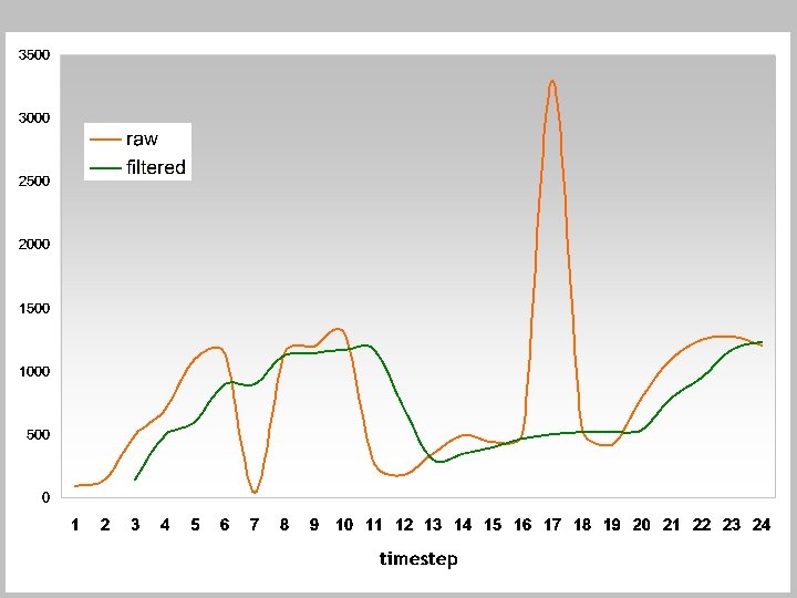
Minimizing noise • cloud/shadow best: detection and interpolation for now: median temporal filtering

Minimizing noise • cloud/shadow best: detection and interpolation for now: median temporal filtering • variability in veg phenology and soil background best: score standardization by forest type group for now: " " "
")
Forest type groups Brewer et al. (2005)

Image standardization landcover classes imagery outlier excerpt one class standardize imagery

Minimizing noise • cloud/shadow best: detection and interpolation for now: median temporal filtering • variability in veg phenology and soil background best: score standardization by forest type group for now: " " " • atmospheric variability best: score standardization by date for now: spatial high-pass filtering

Minimizing noise • cloud/shadow best: detection and interpolation for now: median temporal filtering • variability in veg phenology and soil background best: score standardization by forest type group for now: " " " • atmospheric variability best: score standardization (need JD for composites) for now: spatial high-pass filtering • view angle best: minimize view angle, use BRDF correction not bad: score standardization by view angle and forest type group for now: spatial high-pass filtering

Establish baseline The real data to be analyzed in all the previous steps are departures from expected values (of reflectance, NDVI, etc. ), rather than the measured values themselves. Best method: form time-series using temporal smoothing of pixel measurements during a year without disturbance • need good survey data and flexible analysis environment For now: try two methods to get baseline reflectances • for each timestep, use reflectances corresponding to year with maximum NDVI • use median value for timestep over all previous years

baseline phenology movie

Conceptual test 1. calculate NDVI from MODIS 16 -day red and NIR reflectances (all further steps done separately for red, NIR, and NDVI) 2. standardize each pixel relative to its forest type group 3. expected values = median of previous years for timestep 4. deviations (red, NIR, NDVI) = current value – expected value 5. 11 x 11 pixel high-pass filter 6. temporal median filter 7. reflectance anomaly score = abs(red score) + abs(NIR score) 8. find maximum yearly anomaly scores for each pixel 9. compare anomaly scores to Landsat forest change maps

Conceptual test NACP forest disturbance, ~1984 -2005

real-time anomaly detection movie

NACP disturbance yr. persisting forest 2004 -2005 2002 -2003 2001 or earlier

2004 -2005 minimum NDVI anomaly

Conceptual test NACP forest disturbance, ~1984 -2005
")
Forest disturbance, 2003 -2004 (Befort)

2003 -2004 minimum NDVI anomaly

So… • It appears so far from our PNW and Hurricane Dean work that collection 5 isn’t going to make the problems in 8 -day composites caused by cloud cover, variability in atmospheric conditions (and view angle) go away. Likewise, the situation with incorrect identification of bad data in the QA info does not seem improved. 16 -day composites may be better, but are not frequent enough for us in operational terms. • The variability in the composites are large compared to the forest signals we’re trying to detect, and there is too much missing data (at least in mountains and humid areas). • We have gotten the idea that we can make better composites (for our purposes) by ourselves, based on MOD 02 or MOD 09 single -date products.
 has a chance of seeing things")
AWi. FS ? • 56 m resolution (vis/NIR/SWIR) has a chance of seeing things that aren’t obvious to everyone already • repeat up to every 5 days has a chance of seeing things before they’re common knowledge and while they can still be acted on • USDA buying in bulk free to USFS
")
MODIS post-tornado (b 721)
")
AWi. FS post-tornado (b 432)
 – September, 24 day")
FY 2007 US Standing Order for AWi. FS April (June) – September, 24 day repeat cycle # acquisitions / 24 days

Next steps • continue with MODIS 8 -day composite and custom composite image tests against FHM data • investigate combination of 1 km BRDF-corrected MODIS data with 250 m standard reflectance composites • examine 2007 AWi. FS data
93b4f5a0859d5f3730c29d2142f6d8b9.ppt