Foreign trade In the next two lectures

Foreign trade • In the next two lectures we will develop versions of the IS-LM and AD-AS models for an open economy. • An open economy can have several meanings: – Goods market: trades goods and services – Financial market: allow the flow of investment capital – Factor market: allows the free movement of companies and people • In this class we will focus on the first two: openness in goods and financial markets.

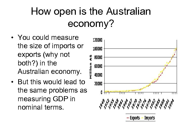How open is the Australian economy? • You could measure the size of imports or exports (why not both? ) in the Australian economy. • But this would lead to the same problems as measuring GDP in nominal terms.

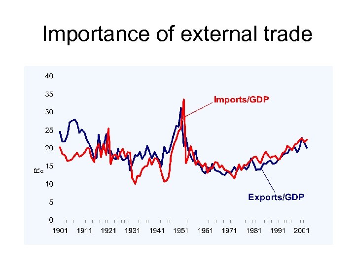Importance of external trade

Globalization? • Much is made of the “new” impact of globalization in the world economy. • But from the previous graph, the Australian economy is as dependent (even less) on the rest of the world as it was one century ago. • “Globalization” must be referring to something else instead- the free flow of people and ideas across the world- rather than goods and services.

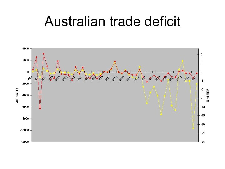
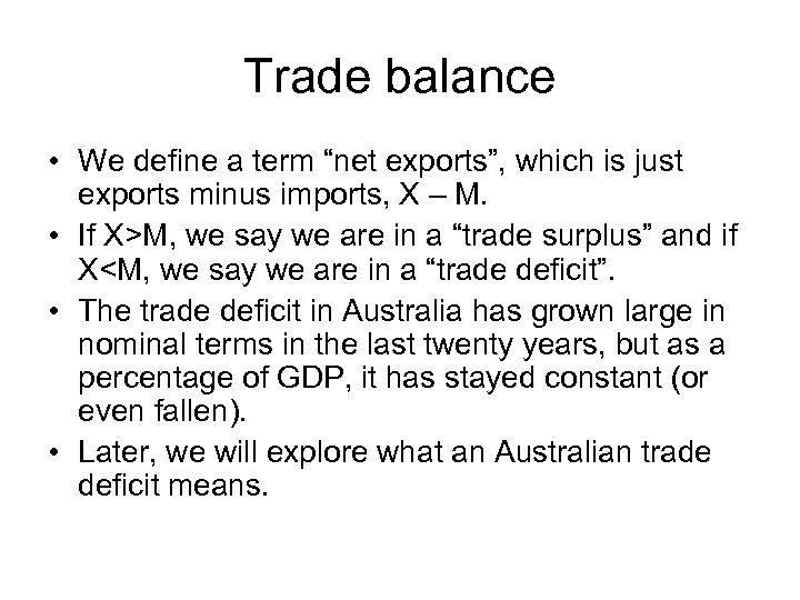Trade balance • We define a term “net exports”, which is just exports minus imports, X – M. • If X>M, we say we are in a “trade surplus” and if X

Australian trade deficit

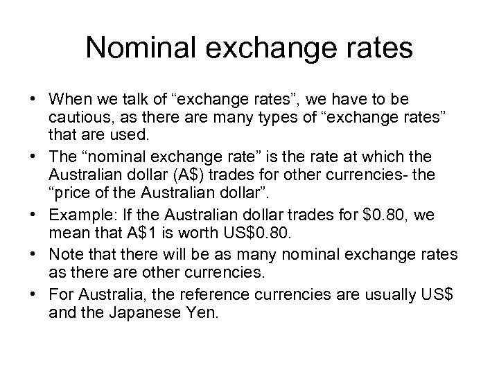Nominal exchange rates • When we talk of “exchange rates”, we have to be cautious, as there are many types of “exchange rates” that are used. • The “nominal exchange rate” is the rate at which the Australian dollar (A$) trades for other currencies- the “price of the Australian dollar”. • Example: If the Australian dollar trades for $0. 80, we mean that A$1 is worth US$0. 80. • Note that there will be as many nominal exchange rates as there are other currencies. • For Australia, the reference currencies are usually US$ and the Japanese Yen.

Price of the A$

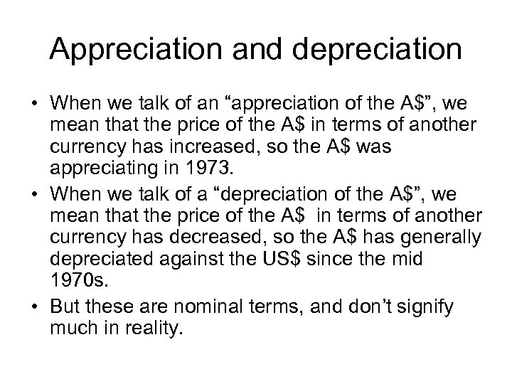Appreciation and depreciation • When we talk of an “appreciation of the A$”, we mean that the price of the A$ in terms of another currency has increased, so the A$ was appreciating in 1973. • When we talk of a “depreciation of the A$”, we mean that the price of the A$ in terms of another currency has decreased, so the A$ has generally depreciated against the US$ since the mid 1970 s. • But these are nominal terms, and don’t signify much in reality.

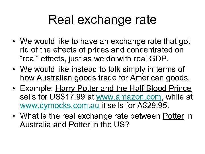Real exchange rate • We would like to have an exchange rate that got rid of the effects of prices and concentrated on “real” effects, just as we do with real GDP. • We would like instead to talk simply in terms of how Australian goods trade for American goods. • Example: Harry Potter and the Half-Blood Prince sells for US$17. 99 at www. amazon. com, while at www. dymocks. com. au it sells for A$29. 95. • What is the real exchange rate between Potter in Australia and Potter in the US?

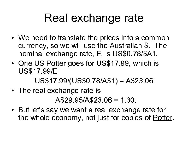Real exchange rate • We need to translate the prices into a common currency, so we will use the Australian $. The nominal exchange rate, E, is US$0. 78/$A 1. • One US Potter goes for US$17. 99, which is US$17. 99/E US$17. 99/(US$0. 78/A$1) = A$23. 06 • The real exchange rate is A$29. 95/A$23. 06 = 1. 30. • But let’s say we want a real exchange rate for the whole economy, not just for copies of Potter.

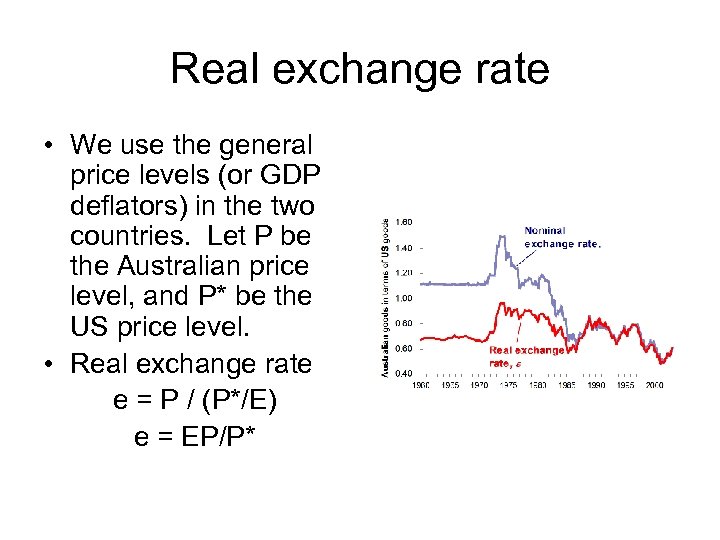Real exchange rate • We use the general price levels (or GDP deflators) in the two countries. Let P be the Australian price level, and P* be the US price level. • Real exchange rate e = P / (P*/E) e = EP/P*

Real exchange rate • The real exchange rate then expresses how average prices are moving in Australia with respect to other countries, such as the US. • The nominal exchange rate of the A$, E, fell against the US$, but the real exchange rate did not fall as much. Why? • Answer: Average inflation in Australia was higher than in the US, so P grew faster than P* balancing out the drop in E.

Multilateral exchange rates • The higher is e, the cheaper US goods are compared to Australian goods. • So far we have been considering only exchange rates between Australia and the US, but Australia trades with many countries. What if the A$ falls against the US$, but rises against the Japanese Yen? • Multilateral exchange rates show the price of the A$ compared to a weighted average of the currencies of our trading partners, where the weight of a currency depends on the percentage of our trade it composes.

What determines E? • The nominal exchange rate (say US$/A$) is determined in a market for A$, where you have both supply and demand for A$. E is the price in this market. • Who demands A$? – Exporters who buy Australian goods to sell overseas. – Foreign investors who buy Australian assets. • Who supplies A$? – Importers who want to buy overseas goods. – Australian investors who buy foreign assets.

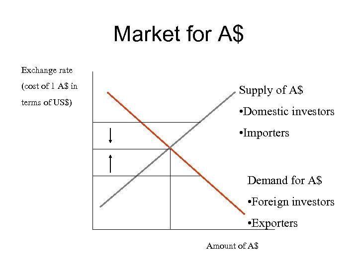Market for A$ Exchange rate (cost of 1 A$ in terms of US$) Supply of A$ • Domestic investors • Importers Demand for A$ • Foreign investors • Exporters Amount of A$

Market for A$ • The nominal exchange rate is then affected both by changes in the goods market and also the financial markets. • But the volume of A$ traded on the world financial markets was A$75 billion per day in 2001, while the volume of goods trade was A$0. 7 per day in 2001. Goods trade was only 1% of financial trading in the A$. • In the short-term, the price of the A$ is determined by changes in financial markets.

Financial market openness • Openness in financial markets means that investors are free to put their money where they wish. • Australian investors are free to invest overseas, and foreign investors are free to invest in Australia. • In this case, investors will put their money where they think it will earn the highest returns. • In equilibrium that means that expected asset returns must be the same in Australia as overseas.

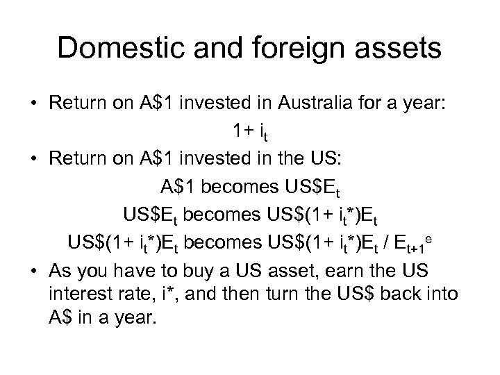Domestic and foreign assets • Return on A$1 invested in Australia for a year: 1+ it • Return on A$1 invested in the US: A$1 becomes US$Et becomes US$(1+ it*)Et / Et+1 e • As you have to buy a US asset, earn the US interest rate, i*, and then turn the US$ back into A$ in a year.

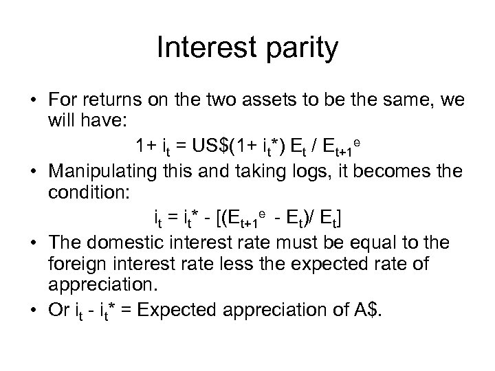Interest parity • For returns on the two assets to be the same, we will have: 1+ it = US$(1+ it*) Et / Et+1 e • Manipulating this and taking logs, it becomes the condition: it = it* - [(Et+1 e - Et)/ Et] • The domestic interest rate must be equal to the foreign interest rate less the expected rate of appreciation. • Or it - it* = Expected appreciation of A$.

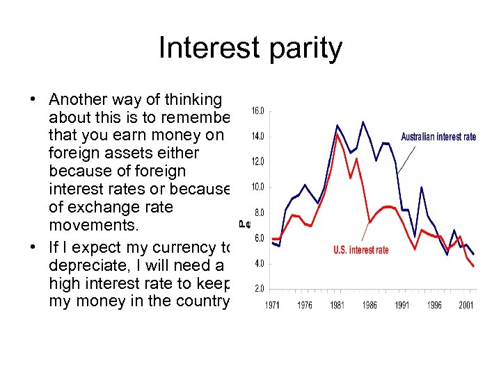Interest parity • Another way of thinking about this is to remember that you earn money on foreign assets either because of foreign interest rates or because of exchange rate movements. • If I expect my currency to depreciate, I will need a high interest rate to keep my money in the country.

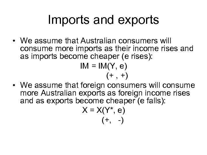Imports and exports • We assume that Australian consumers will consume more imports as their income rises and as imports become cheaper (e rises): IM = IM(Y, e) (+ , +) • We assume that foreign consumers will consume more Australian exports as foreign income rises and as exports become cheaper (e falls): X = X(Y*, e) (+, -)

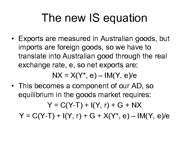The new IS equation • Exports are measured in Australian goods, but imports are foreign goods, so we have to translate into Australian good through the real exchange rate, e, so net exports are: NX = X(Y*, e) – IM(Y, e)/e • This becomes a component of our AD, so equilibrium in the goods market requires: Y = C(Y-T) + I(Y, r) + G + NX Y = C(Y-T) + I(Y, r) + G + X(Y*, e) – IM(Y, e)/e

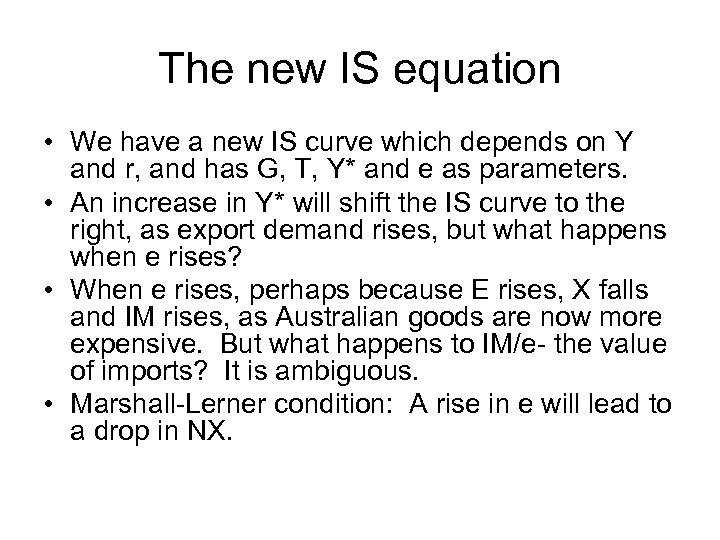The new IS equation • We have a new IS curve which depends on Y and r, and has G, T, Y* and e as parameters. • An increase in Y* will shift the IS curve to the right, as export demand rises, but what happens when e rises? • When e rises, perhaps because E rises, X falls and IM rises, as Australian goods are now more expensive. But what happens to IM/e- the value of imports? It is ambiguous. • Marshall-Lerner condition: A rise in e will lead to a drop in NX.

The J curve • Typically prices move much faster than goods supply and demand- ie. firms order goods in advance. • In this case, X and IM will not move when e falls. But that means that NX will initially fall if e falls, even if the Marshall-Lerner condition is satisfied. Eventually however the X and IM will react and NX will rise. • We saw this in the early 80 s in Australia.

Paul Keating’s J curve