Forecasting of Demand Chapter 7 of Chopra Read

Forecasting of Demand Chapter 7 of Chopra Read: Chap. 7. 1 -7. 4; p 207; p 212 -214 (upto/exclude “Trend-corrected …”); 7. 6; 7. 7 -upto p 220 (exclude “Trend-corrected …”); 7. 10. 1

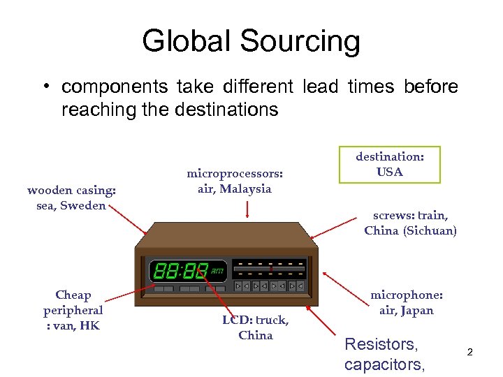Global Sourcing • components take different lead times before reaching the destinations wooden casing: sea, Sweden Cheap peripheral : van, HK microprocessors: air, Malaysia destination: USA screws: train, China (Sichuan) LCD: truck, China microphone: air, Japan Resistors, capacitors, 2

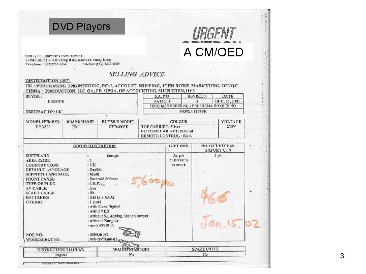DVD Players A CM/OED 3

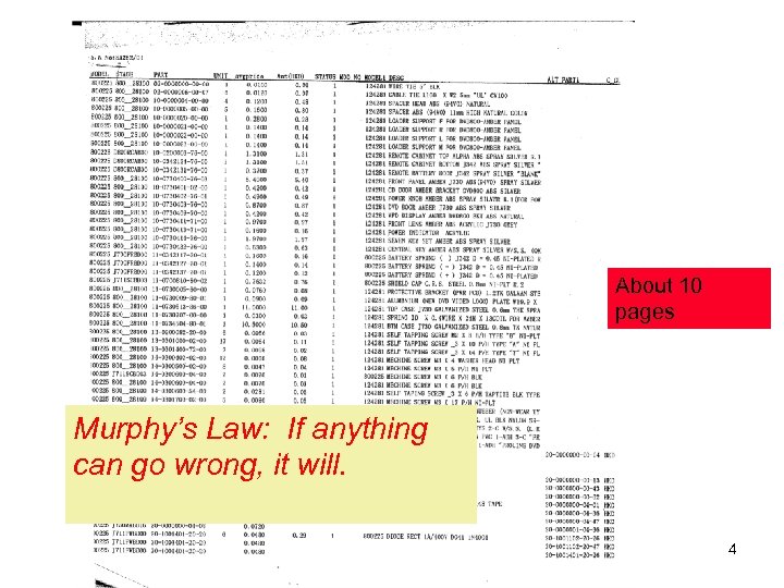About 10 pages Murphy’s Law: If anything can go wrong, it will. 4

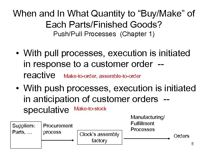When and In What Quantity to “Buy/Make” of Each Parts/Finished Goods? Push/Pull Processes (Chapter 1) • With pull processes, execution is initiated in response to a customer order -reactive Make-to-order, assemble-to-order • With push processes, execution is initiated in anticipation of customer orders -speculative Make-to-stock Suppliers: Parts, … Procurement process Clock’s assembly factory Manufacturing/ Fulfillment Processes Orders 5

Learning Objectives • • Describe types of forecasts Describe time series Use time series forecasting methods Explain how to monitor & control forecasts 6

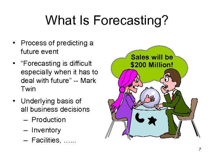What Is Forecasting? • Process of predicting a future event • “Forecasting is difficult especially when it has to deal with future” -- Mark Twin Sales will be $200 Million! • Underlying basis of all business decisions – Production – Inventory – Facilities, …. . . 7

Why forecast demand? • We need to know how much to make ahead of time, i. e. our production schedule – How much raw material – How many workers – How much to ship to the warehouse in XXX • We need to know how much production capacity to build 8

Why Forecasting ? • You’re managing merchandises for Park’n Shop. Fruits take 3 wks to arrive from Australia. • You need to commit to a number of containers NOW for the month of March in order for a better price • Coca-Cola Bottling: next quarter’s demand + promotions -> production plan/ orders of concentrates 9

Forecasting is Always Wrong • “I think there is a world mkt for maybe 5 computers” Thomas Watson, Chairman of IBM, 1955 • “There is no reason anyone would want a computer in their home. ” - Ken Olson, CEO and Founder of Digital Equipment Corp. , 1977 • “ 640 K should be enough for anybody. ” -- Bill Gates, 1981 • “Economists are good at explaining why their forecasts always went wrong” -- Economist, xx, 1998 • “Fore. represents a constant pain for human being” -- some one 10

Coping with Forecast Errors • Better forecasting methods (e. g. , new SCM concepts) • Buffer mechanism (e. g. , safety stock) • Shorter lead time (i. e. , reducing f horizon) • Flexible ops (mass customisation approach) 11

Forecasting v. s. Planning • Forecast: – About what will happen in future • Plan: – About what should happen in future – Forecasts as input • All plans are based upon some fore. explicitly or implicitly 12

Forecasting v. s. Planning • When sales dept. shows sales forecasts, be cautious. They may be goals • Both forecasting and planning are art and science – Quant f methods - educated guessing • must be tempered by judgement bec’s • quant f assumes future is a continuation of the past 13

Types of Forecasts by Time Horizon • Short-range forecast – Up to 1 year; usually < 3 months – Procurement, worker assignments • Medium-range forecast – 3 months to 3 years – Sales & production planning, budgeting • Long-range forecast – 3 + years – Capacity planning, facility location 14

15

Types of Forecasts by Item Forecast • Key forecasts in business: • Future demand for products, Sales • Demand (sales = demand - lost sales) • Future price of various commodities • Lead times • Processing times (learning curves) … 16

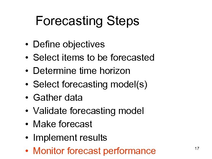Forecasting Steps • • • Define objectives Select items to be forecasted Determine time horizon Select forecasting model(s) Gather data Validate forecasting model Make forecast Implement results Monitor forecast performance 17

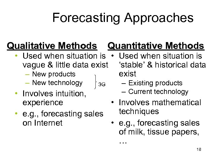Forecasting Approaches Qualitative Methods Quantitative Methods • Used when situation is vague & little data exist ‘stable’ & historical data – New products exist – New technology 3 G – Existing products – Current technology • Involves intuition, experience • Involves mathematical techniques • e. g. , forecasting sales on Internet • e. g. , forecasting sales of milk, tissue papers, … 18

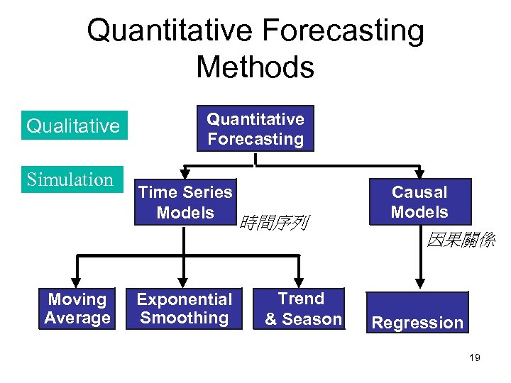Quantitative Forecasting Methods Qualitative Simulation Moving Average Quantitative Forecasting Time Series Models Exponential Smoothing 時間序列 Trend & Season Causal Models 因果關係 Regression 19 A future is continuation of the past (short run)

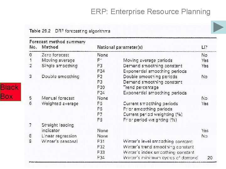ERP: Enterprise Resource Planning Black Box 20

What’s a Time Series? • Set of evenly spaced numerical data – Obtained by observing response variable at regular time periods • Forecast based only on past values – Assumes that factors influencing past, present, & future will continue 21

1 st & 2 nd Law of Forecasting 1. In forecasting, we assume the future will behave like the past – If behavior changes, our forecasts can be terrible 2. Even given 1, there is a limit to how accurate forecasts can be (or nothing can be predicted with complete accuracy) – The achievable accuracy depends on the magnitude of the noise component 22

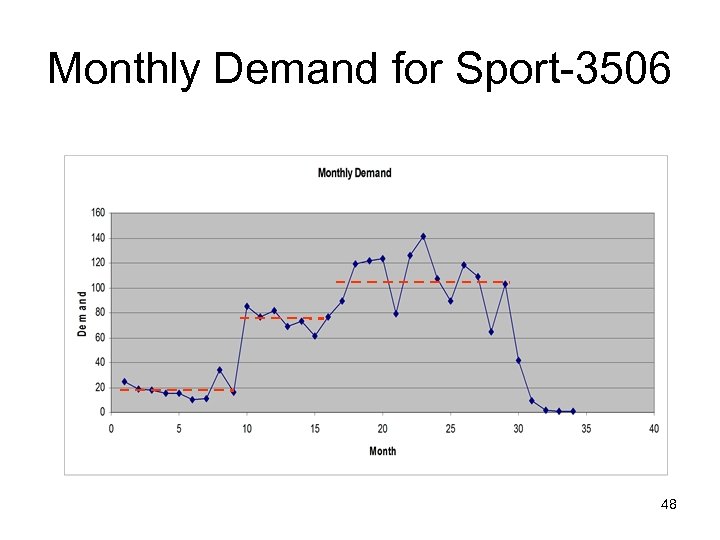
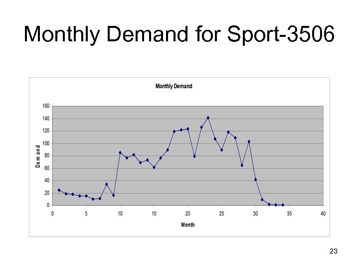Monthly Demand for Sport-3506 23

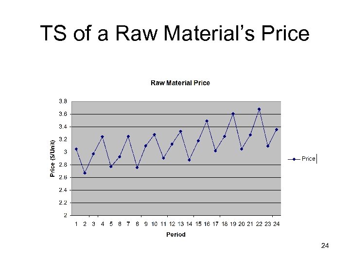TS of a Raw Material’s Price 24

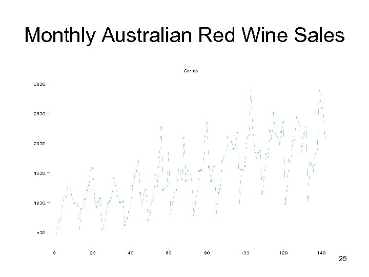Monthly Australian Red Wine Sales 25

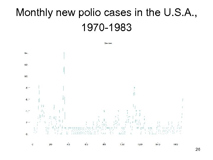Monthly new polio cases in the U. S. A. , 1970 -1983 26

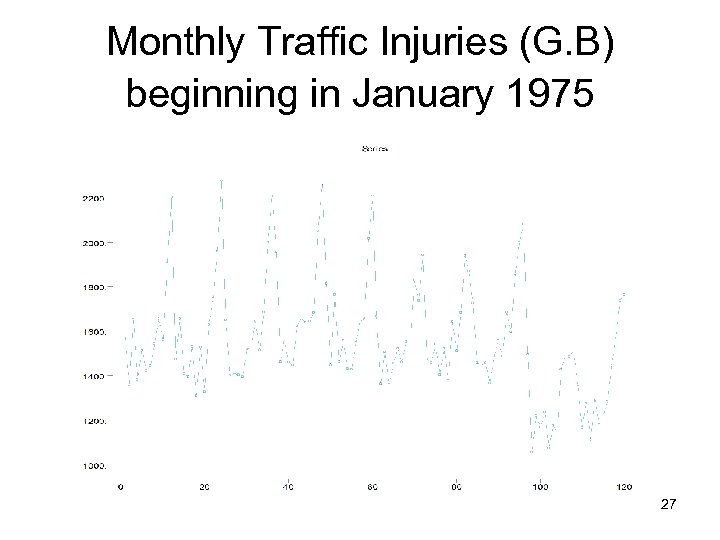Monthly Traffic Injuries (G. B) beginning in January 1975 27

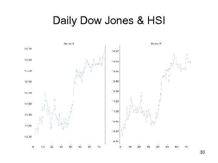Daily Dow Jones & HSI 30

Time Series Components Sales Original T. S. Time 31

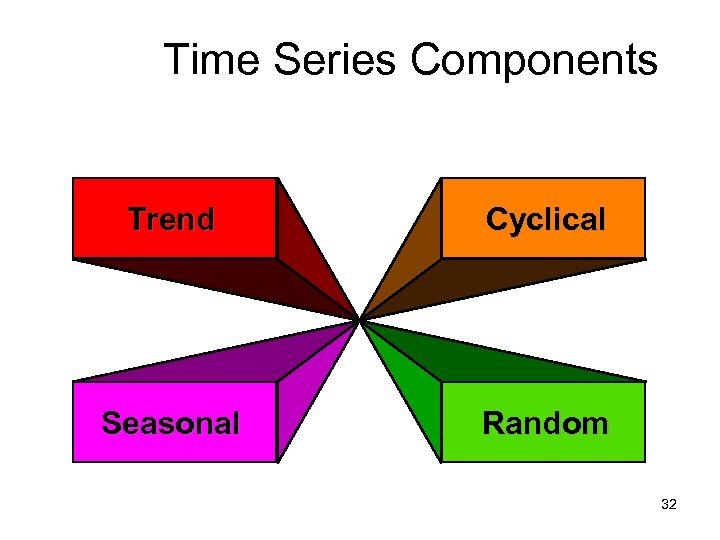Time Series Components Trend Cyclical Seasonal Random 32

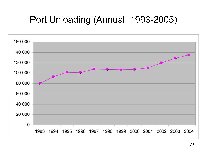
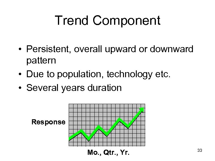Trend Component • Persistent, overall upward or downward pattern • Due to population, technology etc. • Several years duration Response Mo. , Qtr. , Yr. 33

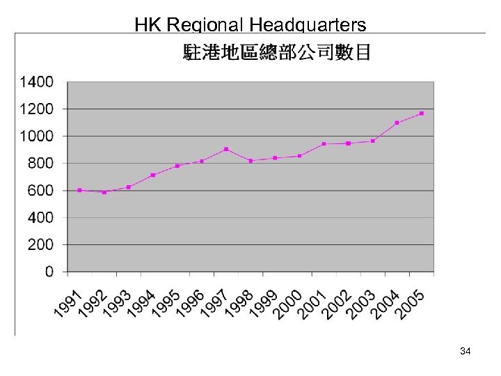HK Regional Headquarters 34

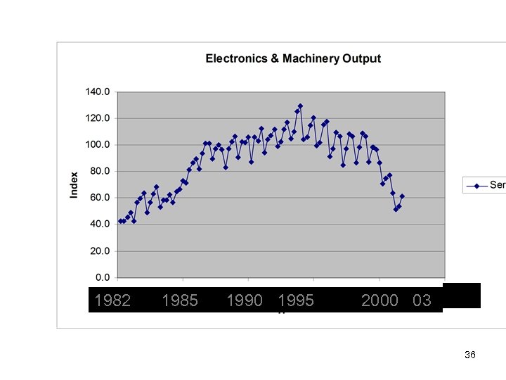
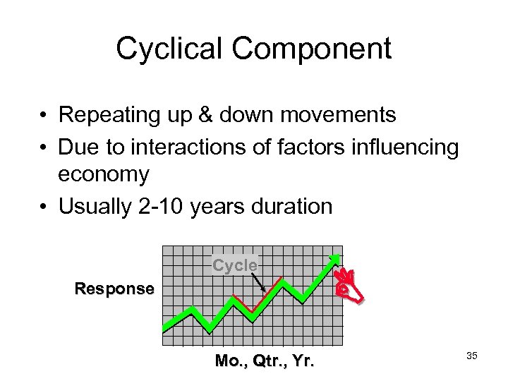Cyclical Component • Repeating up & down movements • Due to interactions of factors influencing economy • Usually 2 -10 years duration Cycle Response Mo. , Qtr. , Yr. 35

1982 1985 1990 1995 2000 03 36

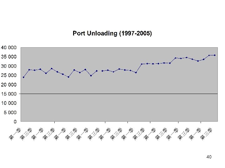
Port Unloading (Annual, 1993 -2005) 37

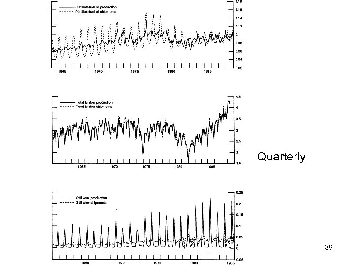
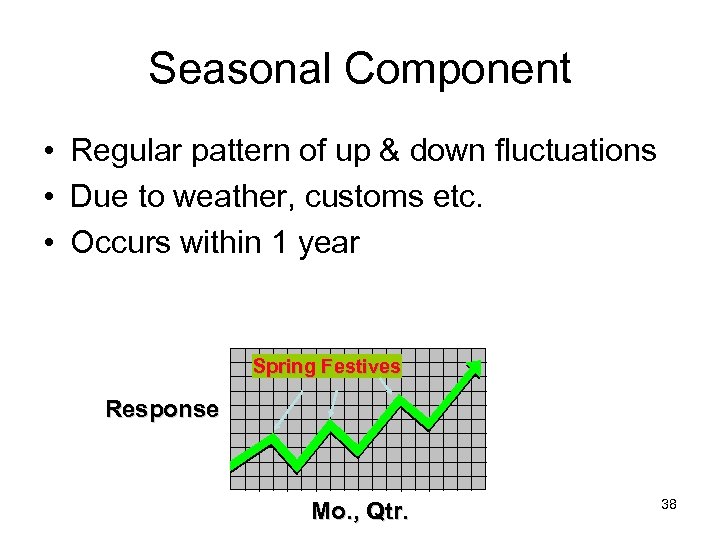Seasonal Component • Regular pattern of up & down fluctuations • Due to weather, customs etc. • Occurs within 1 year Spring Festives Response Mo. , Qtr. 38

Quarterly 39

40

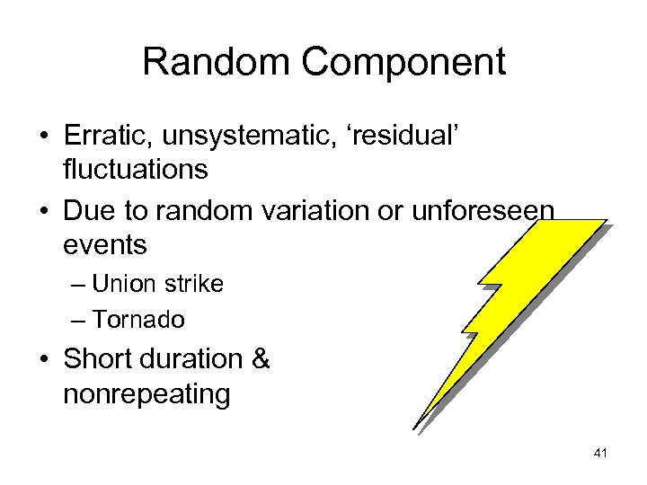Random Component • Erratic, unsystematic, ‘residual’ fluctuations • Due to random variation or unforeseen events – Union strike – Tornado • Short duration & nonrepeating 41

General Time Series Models • Any observed value in a time series is the product (or sum) of time series components • Multiplicative model Yi = Ti · Si · Ci · Ri (if quarterly or mo. data) • Additive model Yi = Ti + Si + Ci + Ri (if quarterly or mo. data) • Hybrids 42

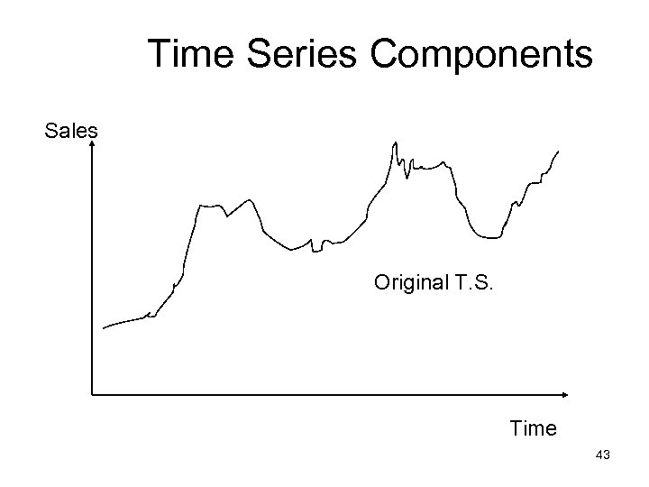Time Series Components Sales Original T. S. Time 43

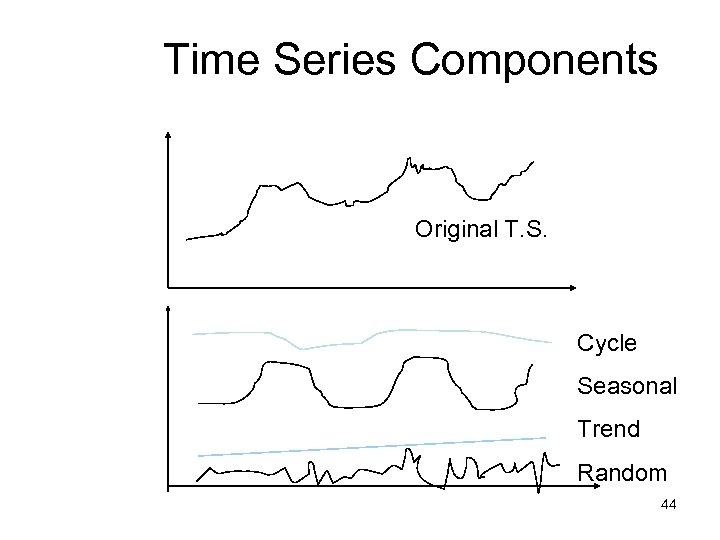Time Series Components Original T. S. Cycle Seasonal Trend Random 44

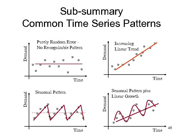Purely Random Error No Recognizable Pattern Demand Sub-summary Common Time Series Patterns Increasing Linear Trend Time Seasonal Pattern Demand Time Seasonal Pattern plus Linear Growth Time 45

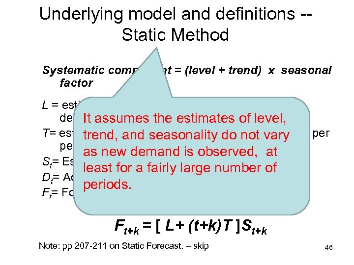Underlying model and definitions -Static Method Systematic component = (level + trend) x seasonal factor L = estimate of level for period 0 (de-seasonalised demand) It assumes the estimates of level, T= estimate of trend seasonality do not vary trend, and (increase/decrease in demand period) as new demand is observed, at St= Estimate of seasonal factor for period t least for a fairly large number of Dt= Actual demand observed for period t periods. Ft= Forecast of demand for period t Ft+k = [ L+ (t+k)T ]St+k Note: pp 207 -211 on Static Forecast. – skip 46

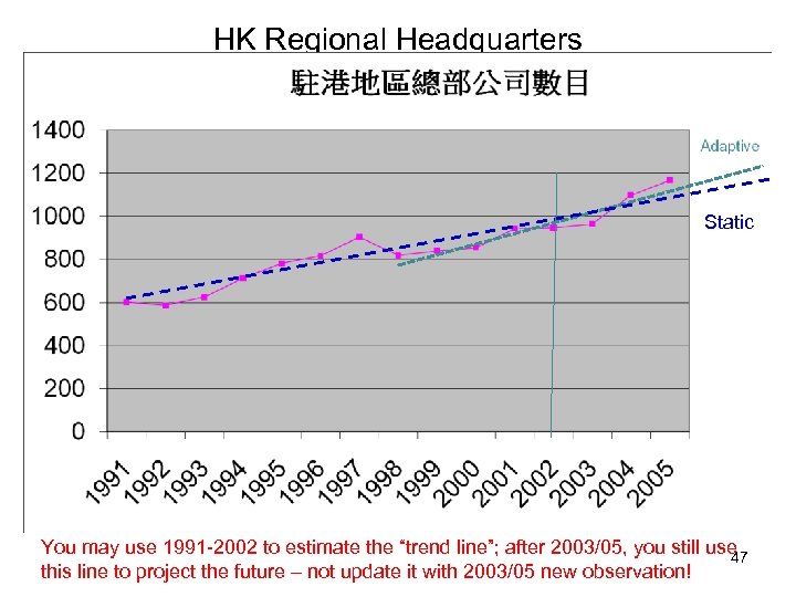HK Regional Headquarters Static You may use 1991 -2002 to estimate the “trend line”; after 2003/05, you still use 47 this line to project the future – not update it with 2003/05 new observation!

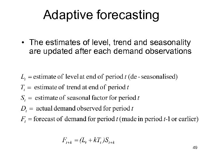
Monthly Demand for Sport-3506 48

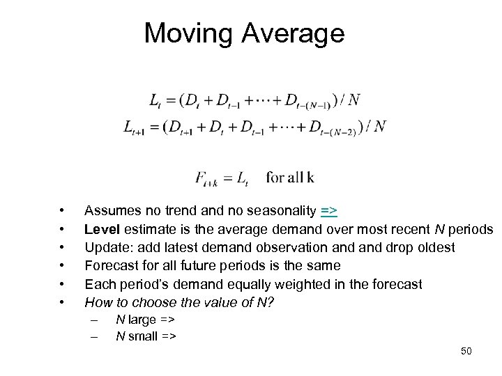
Adaptive forecasting • The estimates of level, trend and seasonality are updated after each demand observations 49

Moving Average • • • Assumes no trend and no seasonality => Level estimate is the average demand over most recent N periods Update: add latest demand observation and drop oldest Forecast for all future periods is the same Each period’s demand equally weighted in the forecast How to choose the value of N? – – N large => N small => 50

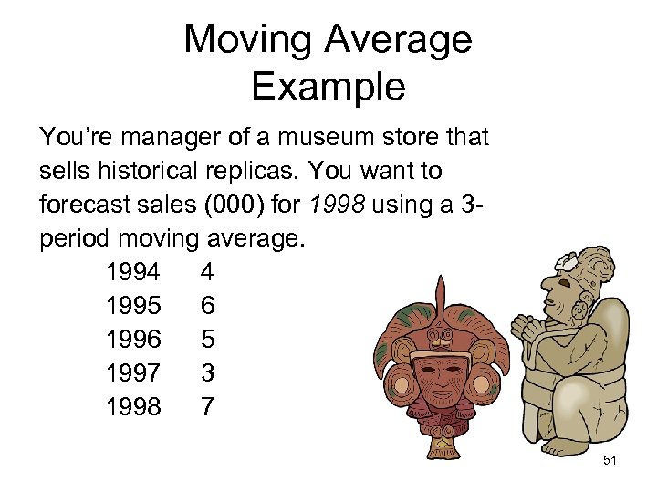Moving Average Example You’re manager of a museum store that sells historical replicas. You want to forecast sales (000) for 1998 using a 3 period moving average. 1994 4 1995 6 1996 5 1997 3 1998 7 51

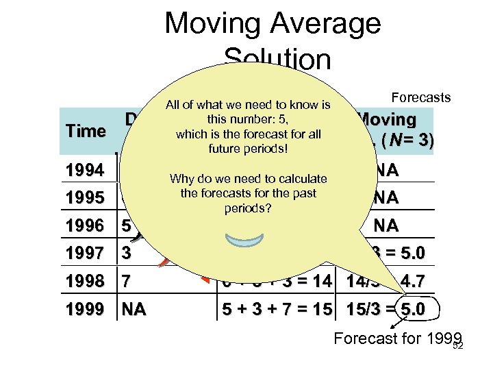Moving Average Solution Time All of what we need to know is Demand this number: 5, Total Moving is the Di which future forecast for all (N = 3) periods! 1994 4 1995 6 1996 5 NA Why do we need NA to calculate the forecasts for the past NA periods? NA Forecasts Moving Avg. ( N = 3) NA NA NA 1997 3 4 + 6 + 5 = 15 15/3 = 5. 0 1998 7 6 + 5 + 3 = 14 14/3 = 4. 7 1999 NA 5 + 3 + 7 = 15 15/3 = 5. 0 Forecast for 1999 52

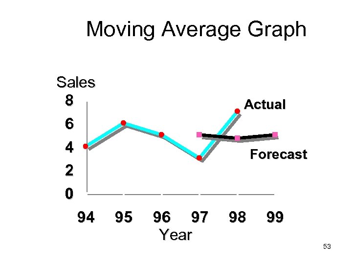Moving Average Graph Sales 8 6 4 2 0 94 Actual Forecast 95 96 97 Year 98 99 53

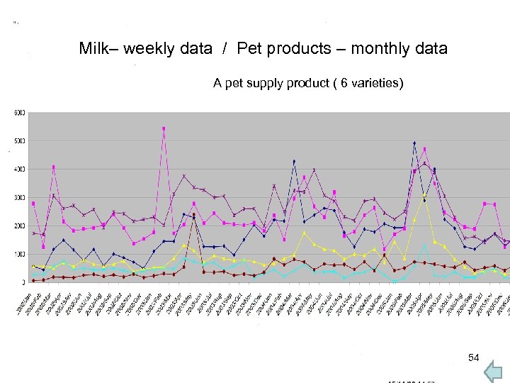Milk– weekly data / Pet products – monthly data A pet supply product ( 6 varieties) 54

Moving Average Method • Used if little or no trend • Used often for smoothing – Provides overall impression of data over time • Why “moving” not just overall mean? 55

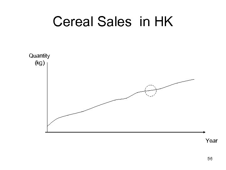Cereal Sales in HK Quantity (kg) Year 56

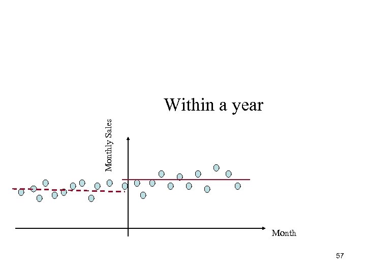Monthly Sales Within a year Month 57

Disadvantages of Moving Averages • Increasing N makes forecast less sensitive to changes • Do not forecast trend well • Require much historical data – N, while exponential only last forecast! 58

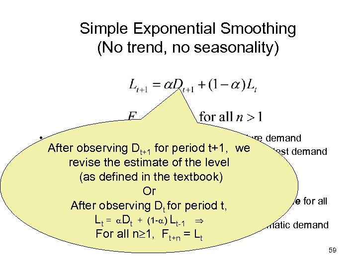Simple Exponential Smoothing (No trend, no seasonality) • Rationale: recent past more indicative of future demand • After observing Dt+1 for weightedt+1, we of latest demand Update: level estimate is period average observation and previous estimate revise the estimate of the level • is called the smoothing textbook) < < 1) (as defined in the constant (0 • Forecast for all future periods is the same Or • Assume systematic component of demand is the same for all After observing Dt for period t, periods (L) Lt = Dt + (1 - ) Lt-1 • Lt is the best guess at period t of what the systematic demand level is For all n 1, Ft+n = Lt 59

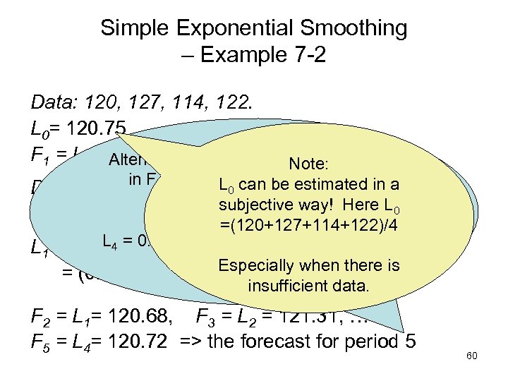Simple Exponential Smoothing – Example 7 -2 Data: 120, 127, 114, 122. L 0= 120. 75 = 0. 1 F 1 = L 0 =120. 75 Alternatively, if you are Note: only interested L can be estimated in D 1= 120 in F 5, then L 30 = (120+127+114)/3 a =120. 33 subjective way! Here L 0 E 1 = F 1 – D 1 = 120. 75 – 120 = 0. 75 =(120+127+114+122)/4 = 0. 1 a ) L L 1 = a DL 4+ (1 - D 4+0. 9 L 3 = 12. 2+108. 2 =120. 4 1 0 Especially = 120. 68 = (0. 1)(120) + (0. 9)(120. 75)when there is => F 5 insufficient data. = 120. 4 F 2 = L 1= 120. 68, F 3 = L 2 = 121. 31, … F 5 = L 4= 120. 72 => the forecast for period 5 60

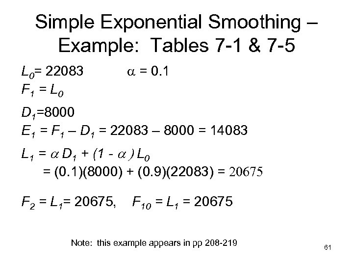Simple Exponential Smoothing – Example: Tables 7 -1 & 7 -5 L 0= 22083 F 1 = L 0 = 0. 1 D 1=8000 E 1 = F 1 – D 1 = 22083 – 8000 = 14083 L 1 = a D 1 + (1 - a ) L 0 = (0. 1)(8000) + (0. 9)(22083) = 20675 F 2 = L 1= 20675, F 10 = L 1 = 20675 Note: this example appears in pp 208 -219 61

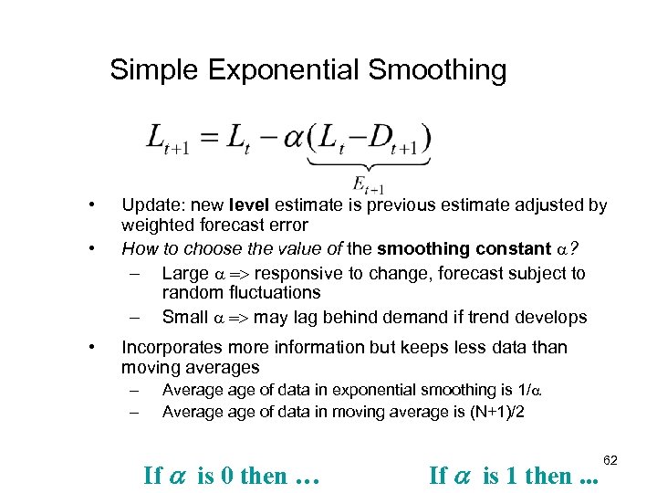Simple Exponential Smoothing • • • Update: new level estimate is previous estimate adjusted by weighted forecast error How to choose the value of the smoothing constant ? – Large => responsive to change, forecast subject to random fluctuations – Small => may lag behind demand if trend develops Incorporates more information but keeps less data than moving averages – – Average of data in exponential smoothing is 1/ Average of data in moving average is (N+1)/2 If a is 0 then … If a is 1 then. . . 62

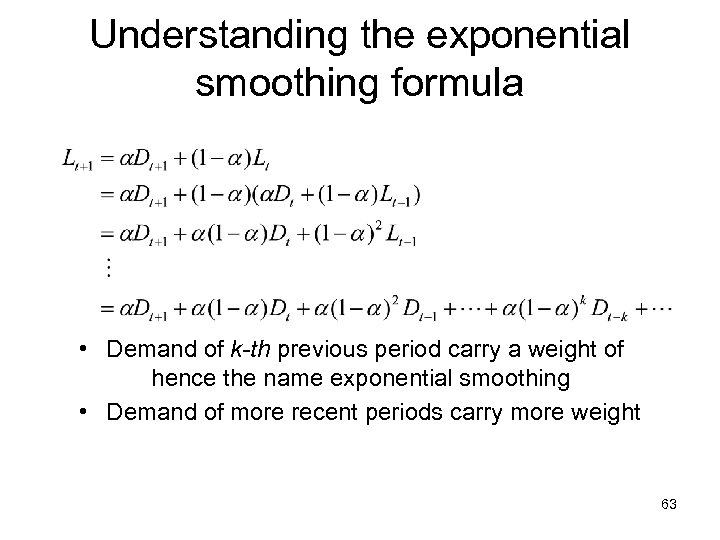Understanding the exponential smoothing formula • Demand of k-th previous period carry a weight of hence the name exponential smoothing • Demand of more recent periods carry more weight 63

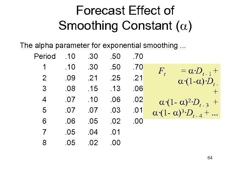Forecast Effect of Smoothing Constant ( ) The alpha parameter for exponential smoothing. . . Period. 10. 30. 50. 70 1. 10. 30. 50. 70 Ft = ·Dt - 1 + 2. 09. 21. 25. 21 ·(1 - )·Dt 3. 08. 15. 13. 06 + 4. 07. 10. 06. 02 ·(1 - )2·Dt - 3 + 5. 07. 03. 01 ·(1 - )3·D t - 4 +. . . 6. 05. 02. 00 7. 05. 04. 01 8. 05. 02. 00 64

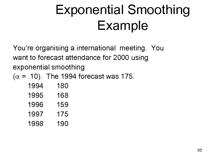Exponential Smoothing Example You’re organising a international meeting. You want to forecast attendance for 2000 using exponential smoothing ( =. 10). The 1994 forecast was 175. 1994 180 1995 168 1996 159 1997 175 1998 190 65

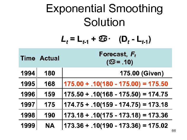Exponential Smoothing Solution Lt = Lt-1 + · (Dt - Lt-1) Time Actual Forecast, Ft ( . 10) = 1994 180 175. 00 (Given) 1995 168 175. 00 +. 10(180 - 175. 00) = 175. 50 1996 159 175. 50 +. 10(168 - 175. 50) = 174. 75 1997 175 174. 75 +. 10(159 - 174. 75) = 173. 18 1998 190 173. 18 +. 10(175 - 173. 18) = 173. 36 1999 NA 173. 36 +. 10(190 - 173. 36) = 175. 02 66

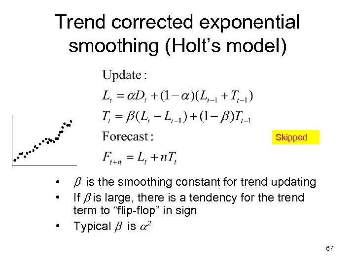Trend corrected exponential smoothing (Holt’s model) Skipped • • • b is the smoothing constant for trend updating If b is large, there is a tendency for the trend term to “flip-flop” in sign Typical b is a 2 67

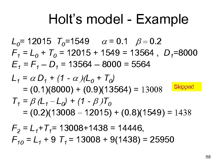Holt’s model - Example L 0= 12015 T 0=1549 a = 0. 1 b = 0. 2 F 1 = L 0 + T 0 = 12015 + 1549 = 13564 , D 1=8000 E 1 = F 1 – D 1 = 13564 – 8000 = 5564 L 1 = a D 1 + (1 - a )(L 0 + T 0) = (0. 1)(8000) + (0. 9)(13564) = 13008 Skipped T 1 = b (L 1 - L 0) + (1 - b )T 0 = (0. 2)(13008 - 12015) + (0. 8)(1549) = 1438 F 2 = L 1+T 1= 13008+1438 = 14446, F 10 = L 1 + 9 T 1 = 13008 + 9(1438) = 25950 68

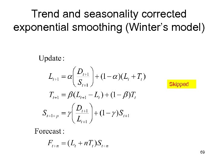Trend and seasonality corrected exponential smoothing (Winter’s model) Skipped 69

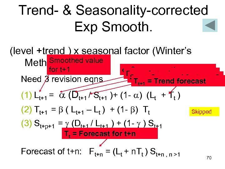Trend- & Seasonality-corrected Exp Smooth. (level +trend ) x seasonal factor (Winter’s Smoothed value Method/Model) for t+1 Need 3 revision eqns D , = smooth. para. , t+1 ST ==Actual forecast p? Seasonal factor, t+1 = Trend t+1 (1) Lt+1 = (Dt+1 / St+1 )+ (1 - ) (Lt + Tt ) (2) Tt+1 = ( Lt+1 – Lt ) + (1 - ) Tt Skipped (3) St+p+1 = (Dt+1 / Lt+1 ) + (1 - ) St+1 Tt = Forecast for t+n Forecast of t+n: Ft+n = (Lt + n. Tt ) St+n , n >1 70

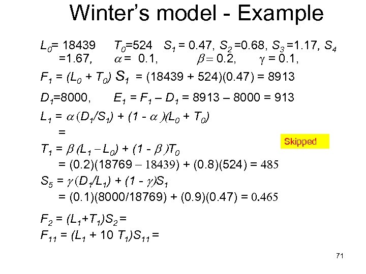Winter’s model - Example L 0= 18439 =1. 67, T 0=524 S 1 = 0. 47, S 2 =0. 68, S 3 =1. 17, S 4 a = 0. 1, b = 0. 2, = 0. 1, F 1 = (L 0 + T 0) S 1 = (18439 + 524)(0. 47) = 8913 D 1=8000, E 1 = F 1 – D 1 = 8913 – 8000 = 913 L 1 = a (D 1/S 1) + (1 - a )(L 0 + T 0) = T 1 = b (L 1 - L 0) + (1 - b )T 0 = (0. 2)(18769 - 18439) + (0. 8)(524) = 485 S 5 = g (D 1/L 1) + (1 - g)S 1 = (0. 1)(8000/18769) + (0. 9)(0. 47) = 0. 465 Skipped F 2 = (L 1+T 1)S 2 = F 11 = (L 1 + 10 T 1)S 11 = 71

Winter’s ES • Why Dt+1 /St+1? • How to initialize the forecast? • How to choose alpha, beta and gamma values? Skipped • Winter’s method is an extension of Holt’s 72

Special Forecasting Difficulties for Supply Chains • New products and service introductions – – • No past history Use qualitative methods until sufficient data collected Examine correlation with similar products Use a large exponential smoothing constant Lumpy derived demand – – – • Not required Large but infrequent orders Random variations “swamps” trend and seasonality Identify reason for lumpiness and modify forecasts Spatial variations in demand – Separate forecast vs. allocation of total forecasts 78

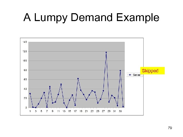A Lumpy Demand Example Skipped 79

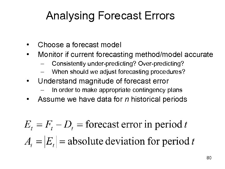Analysing Forecast Errors • • Choose a forecast model Monitor if current forecasting method/model accurate – – • Understand magnitude of forecast error – • Consistently under-predicting? Over-predicting? When should we adjust forecasting procedures? In order to make appropriate contingency plans Assume we have data for n historical periods 80

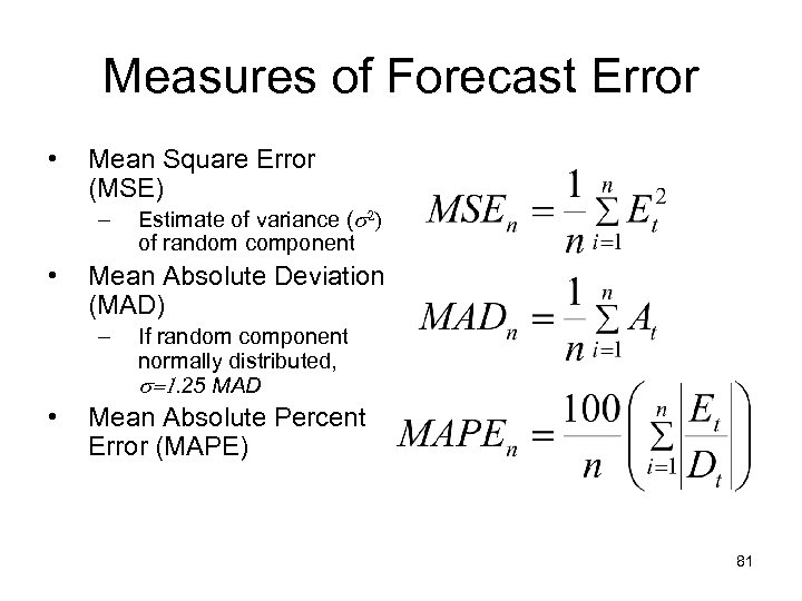Measures of Forecast Error • Mean Square Error (MSE) – • Mean Absolute Deviation (MAD) – • Estimate of variance (s 2) of random component If random component normally distributed, s=1. 25 MAD Mean Absolute Percent Error (MAPE) 81

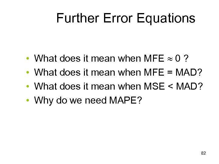Further Error Equations • • What does it mean when MFE 0 ? What does it mean when MFE = MAD? What does it mean when MSE < MAD? Why do we need MAPE? 82

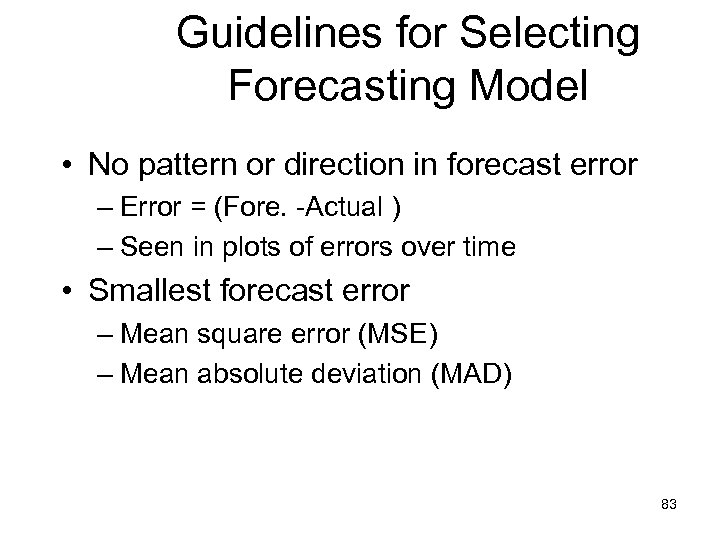Guidelines for Selecting Forecasting Model • No pattern or direction in forecast error – Error = (Fore. -Actual ) – Seen in plots of errors over time • Smallest forecast error – Mean square error (MSE) – Mean absolute deviation (MAD) 83

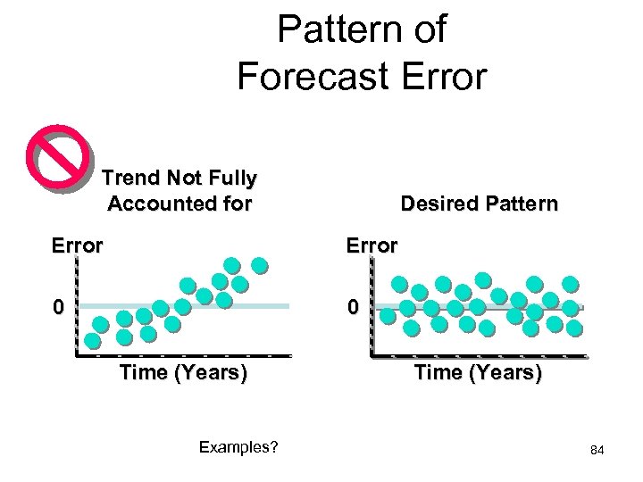Pattern of Forecast Error Trend Not Fully Accounted for Desired Pattern Error 0 0 Time (Years) Examples? Time (Years) 84

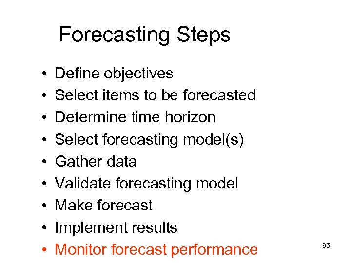Forecasting Steps • • • Define objectives Select items to be forecasted Determine time horizon Select forecasting model(s) Gather data Validate forecasting model Make forecast Implement results Monitor forecast performance 85

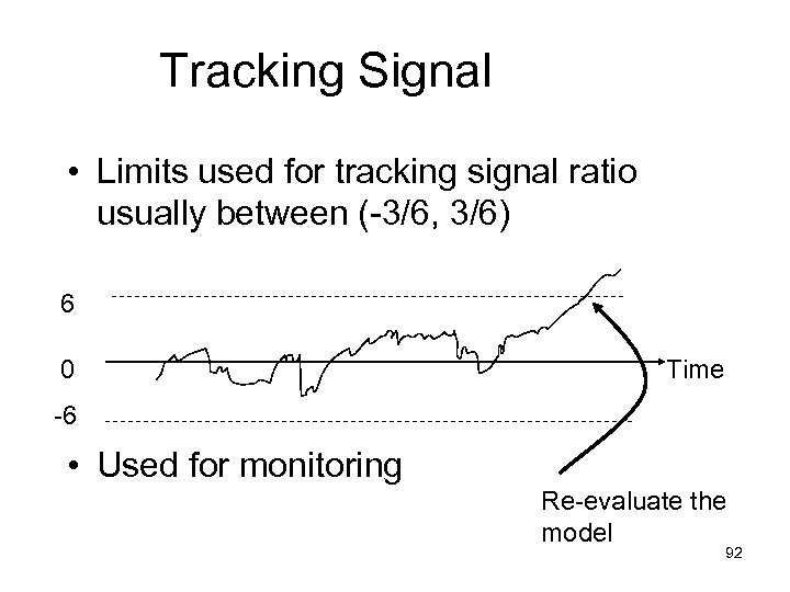
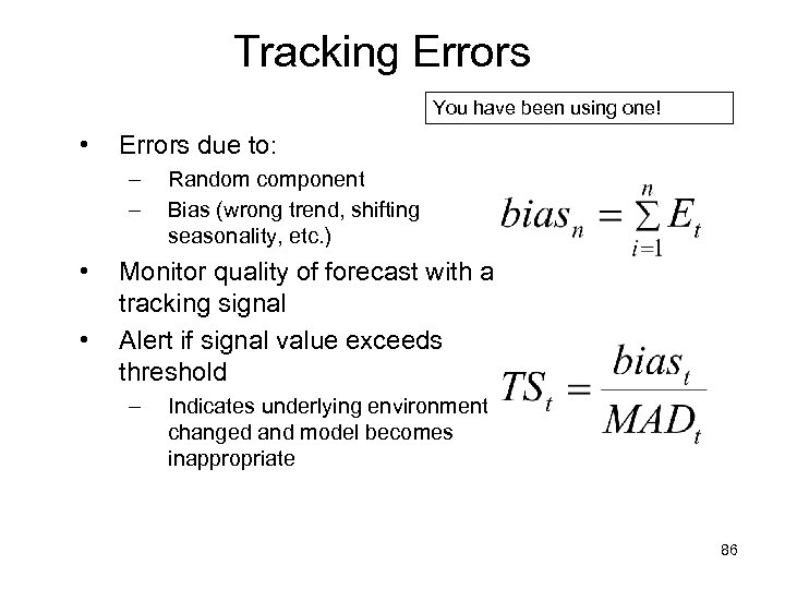Tracking Errors You have been using one! • Errors due to: – – • • Random component Bias (wrong trend, shifting seasonality, etc. ) Monitor quality of forecast with a tracking signal Alert if signal value exceeds threshold – Indicates underlying environment changed and model becomes inappropriate 86

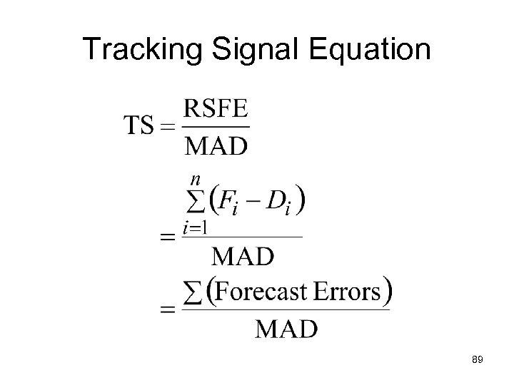
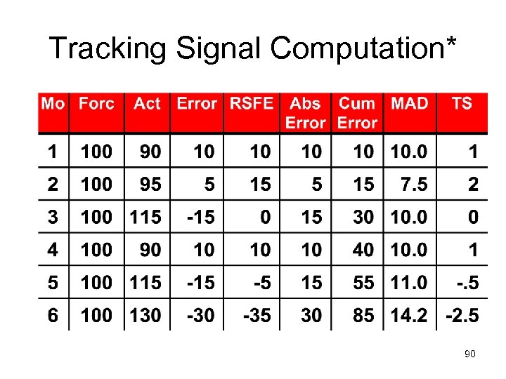
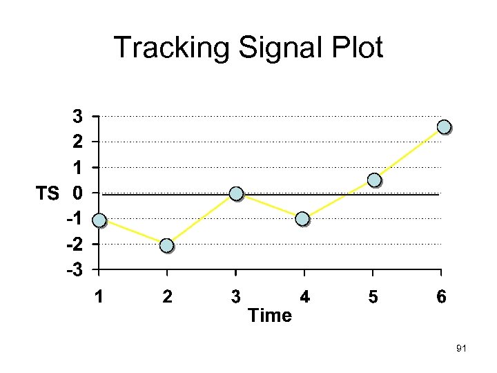
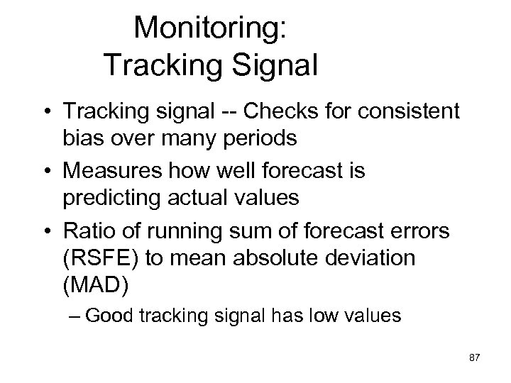Monitoring: Tracking Signal • Tracking signal -- Checks for consistent bias over many periods • Measures how well forecast is predicting actual values • Ratio of running sum of forecast errors (RSFE) to mean absolute deviation (MAD) – Good tracking signal has low values 87

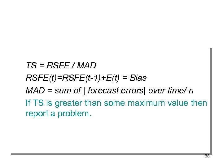TS = RSFE / MAD RSFE(t)=RSFE(t-1)+E(t) = Bias MAD = sum of | forecast errors| over time/ n If TS is greater than some maximum value then report a problem. 88

Tracking Signal Equation 89

Tracking Signal Computation* 90

Tracking Signal Plot 91

Tracking Signal • Limits used for tracking signal ratio usually between (-3/6, 3/6) 6 0 Time -6 • Used for monitoring Re-evaluate the model 92

Tracking Signal • Cautious! – Is it always good to have TS=0? – TS: the smaller the better? – Can TS be used for comparing models? 93

Summary so far • Importance of forecasting in a supply chain • Forecasting models and methods • Exponential smoothing – Stationary model – Trend – Seasonality • Measures of forecast errors • Tracking signals 94

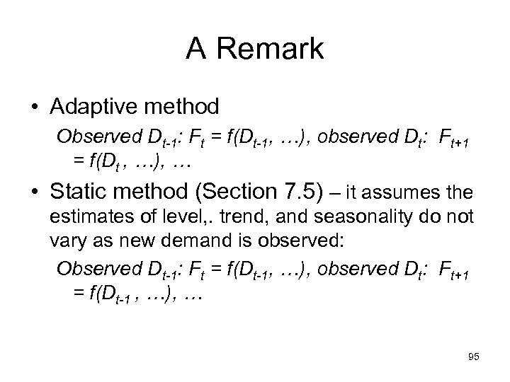A Remark • Adaptive method Observed Dt-1: Ft = f(Dt-1, …), observed Dt: Ft+1 = f(Dt , …), … • Static method (Section 7. 5) – it assumes the estimates of level, . trend, and seasonality do not vary as new demand is observed: Observed Dt-1: Ft = f(Dt-1, …), observed Dt: Ft+1 = f(Dt-1 , …), … 95

• Forget all beyond this slide 96

Part 1 of As# 1 Chapter 7 in 3 rd edition • Discussion questions All are posted as downloadable – Q 4, Q 9 • Exercises – Q 1, Q 2 & Q 3. • The deadline: hand in the class before ? . Part 2 will be released later. 97

Reading List (Chap. 7) • Adaptive Forecasting, up to “Trend- and Seasonality- … Winter’s Model)”. • Section 7. 6. Measures of Forecast Errors. • Section 7. 7, up-to “Trend- and Seasonality - … Winter’s Model)”. 98

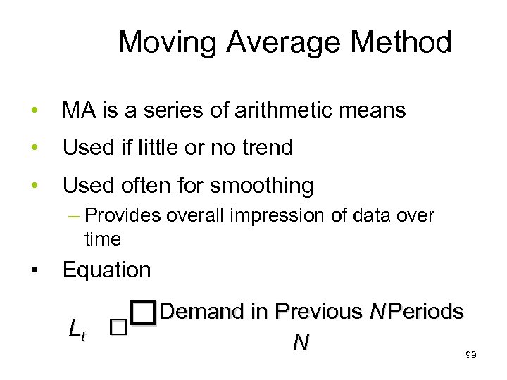Moving Average Method • MA is a series of arithmetic means • Used if little or no trend • Used often for smoothing – Provides overall impression of data over time • Equation Lt Demand in Previous N Periods N 99

Adaptive Forecasting Moving Average Method Systematic component of demand = Level Chopra: p. 82 100

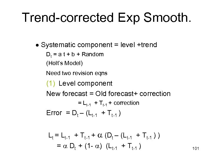Trend-corrected Exp Smooth. Systematic component = level +trend Dt = a t + b + Random (Holt’s Model) Need two revision eqns (1) Level component New forecast = Old forecast+ correction = Lt-1 + Tt-1 + correction Error = Dt – (Lt-1 + Tt-1 ) Lt = Lt-1 + Tt-1 + (Dt – (Lt-1 + Tt-1 ) ) = Dt + (1 - ) (Lt-1 + Tt-1 ) 101

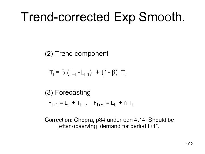Trend-corrected Exp Smooth. (2) Trend component Tt = ( Lt -Lt-1) + (1 - ) Tt (3) Forecasting Ft+1 = Lt + Tt , Ft+n = Lt + n Tt Correction: Chopra, p 84 under eqn 4. 14: Should be “After observing demand for period t+1”. 102

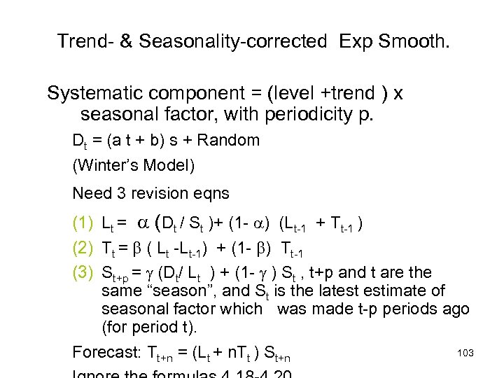Trend- & Seasonality-corrected Exp Smooth. Systematic component = (level +trend ) x seasonal factor, with periodicity p. Dt = (a t + b) s + Random (Winter’s Model) Need 3 revision eqns (1) Lt = (Dt / St )+ (1 - ) (Lt-1 + Tt-1 ) (2) Tt = ( Lt -Lt-1) + (1 - ) Tt-1 (3) St+p = (Dt/ Lt ) + (1 - ) St , t+p and t are the same “season”, and St is the latest estimate of seasonal factor which was made t-p periods ago (for period t). 103 Forecast: Tt+n = (Lt + n. Tt ) St+n

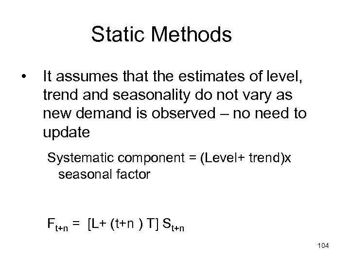Static Methods • It assumes that the estimates of level, trend and seasonality do not vary as new demand is observed – no need to update Systematic component = (Level+ trend)x seasonal factor Ft+n = [L+ (t+n ) T] St+n 104

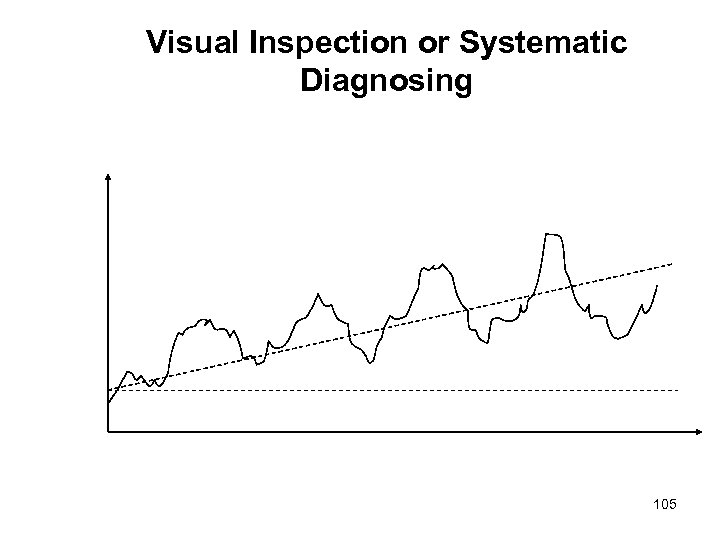Visual Inspection or Systematic Diagnosing 105

Equations fh 106

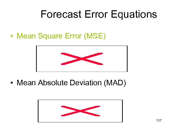Forecast Error Equations • Mean Square Error (MSE) • Mean Absolute Deviation (MAD) 107

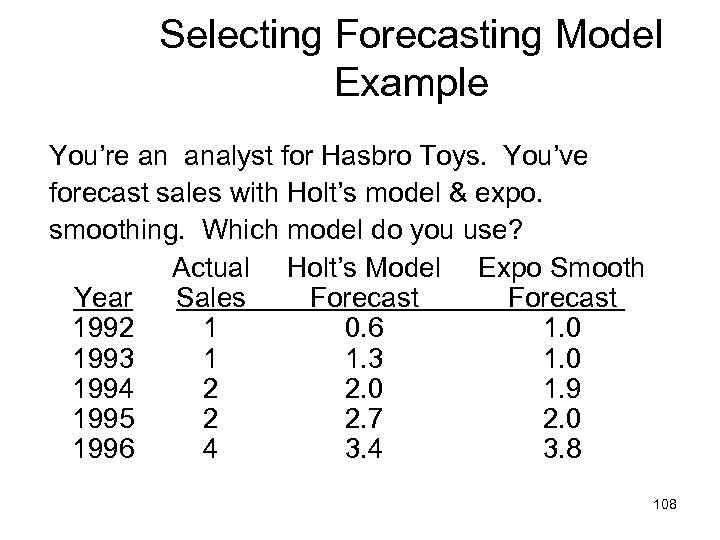Selecting Forecasting Model Example You’re an analyst for Hasbro Toys. You’ve forecast sales with Holt’s model & expo. smoothing. Which model do you use? Actual Holt’s Model Expo Smooth Year Sales Forecast 1992 1 0. 6 1. 0 1993 1 1. 3 1. 0 1994 2 2. 0 1. 9 1995 2 2. 7 2. 0 1996 4 3. 8 108

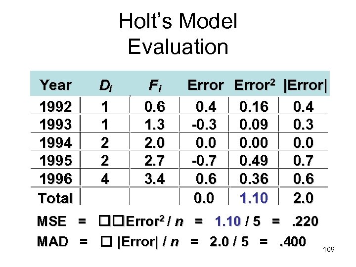Holt’s Model Evaluation Year 1992 1993 1994 1995 1996 Total Di 1 1 2 2 4 Fi 0. 6 1. 3 2. 0 2. 7 3. 4 Error 2 |Error| 0. 4 0. 16 0. 4 -0. 3 0. 09 0. 3 0. 00 0. 0 -0. 7 0. 49 0. 7 0. 6 0. 36 0. 0 1. 10 2. 0 MSE = Error 2 / n = 1. 10 / 5 =. 220 MAD = |Error| / n = 2. 0 / 5 =. 400 109

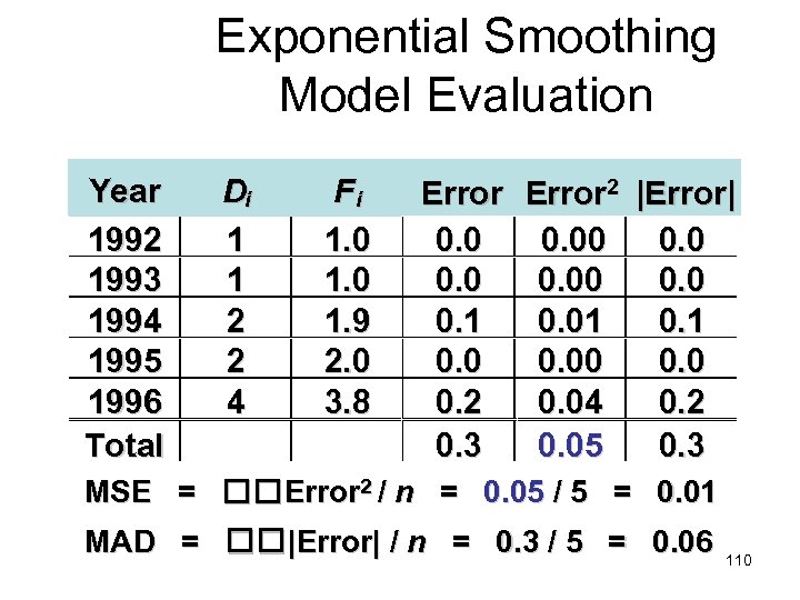Exponential Smoothing Model Evaluation Year 1992 1993 1994 1995 1996 Total Di 1 1 2 2 4 Fi 1. 0 1. 9 2. 0 3. 8 Error 2 |Error| 0. 00 0. 1 0. 01 0. 0 0. 2 0. 04 0. 2 0. 3 0. 05 0. 3 MSE = Error 2 / n = 0. 05 / 5 = 0. 01 MAD = |Error| / n = 0. 3 / 5 = 0. 06 110

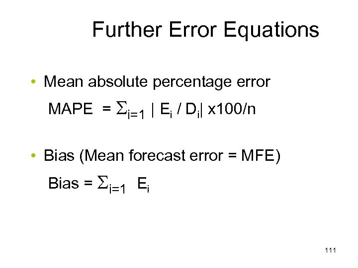Further Error Equations • Mean absolute percentage error MAPE = i=1 | Ei / Di| x 100/n • Bias (Mean forecast error = MFE) Bias = i=1 Ei 111

Further Error Equations • • What does it mean when MFE 0 ? What does it mean when MFE = MAD? What does it mean when MSE < MAD? Why do we need MAPE? 112

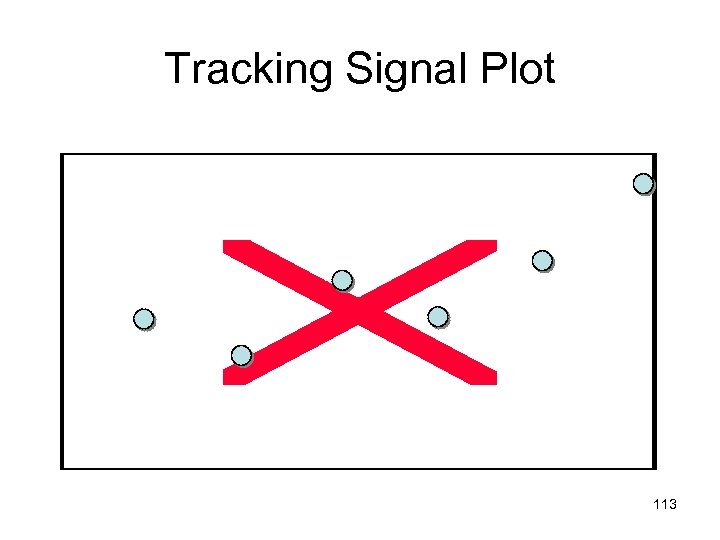Tracking Signal Plot 113

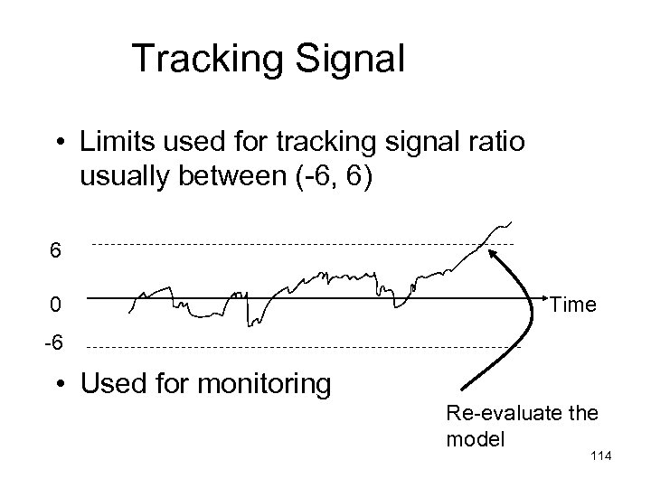Tracking Signal • Limits used for tracking signal ratio usually between (-6, 6) 6 0 Time -6 • Used for monitoring Re-evaluate the model 114

Tracking Signal • Cautious! – Is it always good to have TS=0? – TS: the smaller the better? – Can TS be used for comparing models? 115

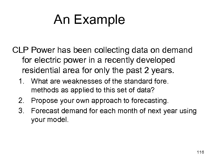An Example CLP Power has been collecting data on demand for electric power in a recently developed residential area for only the past 2 years. 1. What are weaknesses of the standard fore. methods as applied to this set of data? 2. Propose your own approach to forecasting. 3. Forecast demand for each month of next year using your model. 116