Forecasting Interest Rates Structural Models Structural Models

Forecasting Interest Rates Structural Models

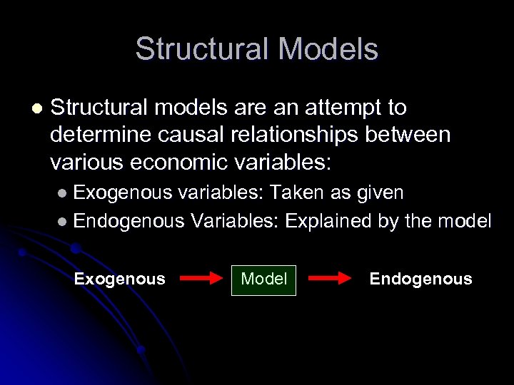Structural Models l Structural models are an attempt to determine causal relationships between various economic variables: l Exogenous variables: Taken as given l Endogenous Variables: Explained by the model Exogenous Model Endogenous

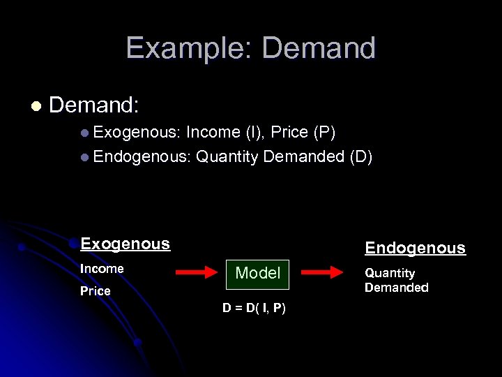Example: Demand l Demand: l Exogenous: Income (I), Price (P) l Endogenous: Quantity Demanded (D) Exogenous Income Endogenous Model Price D = D( I, P) Quantity Demanded

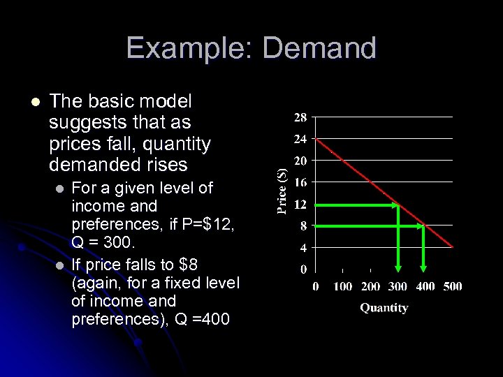Example: Demand l The basic model suggests that as prices fall, quantity demanded rises l l For a given level of income and preferences, if P=$12, Q = 300. If price falls to $8 (again, for a fixed level of income and preferences), Q =400

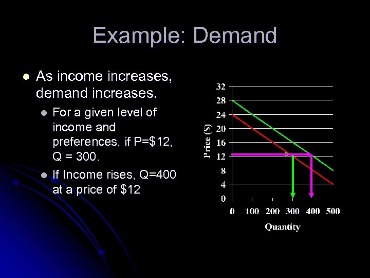Example: Demand l As income increases, demand increases. l l For a given level of income and preferences, if P=$12, Q = 300. If Income rises, Q=400 at a price of $12

Example: Supply l Supply: l Exogenous: Costs (C), Price (P) l Endogenous: Quantity Supplied (S) S = S(C, P)

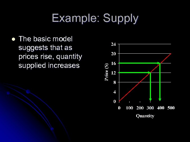Example: Supply l The basic model suggests that as prices rise, quantity supplied increases

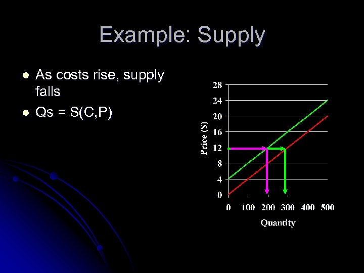Example: Supply l l As costs rise, supply falls Qs = S(C, P)

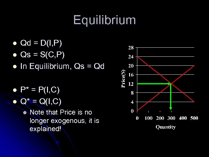Equilibrium l l l Qd = D(I, P) Qs = S(C, P) In Equilibrium, Qs = Qd P* = P(I, C) Q* = Q(I, C) l Note that Price is no longer exogenous, it is explained!

Using Models to Forecast l In the previous example, we ended up with a price equation l. P l The next step would be to estimate the model l. P l = a(C) + b(I) (where a and b are constants) Now, note that the following implies: l P’ l = P(C, I) = a(C’) + b(I’) (‘ indicates a future value) Therefore, to forecast Price: l l l Forecast Costs (C’) Forecast Income (I’) Insert into the estimated price equation to get P’

Interest Rate Models (Real Interest Rates) l Economic models look at how optimizing behavior by households and firms translates into the supply and demand for credit. l Firms choose capital investment projects to maximize shareholder value (Demand) l Households choose consumption/savings to maximize utility (Supply) l Supply = Demand defines the equilibrium interest rate

Household Savings Without an active financial markets, household consumption is restricted to equal current income l With capital markets, the present value of lifetime consumption must equal the present value of lifetime income (assuming all debts are eventually repaid) l

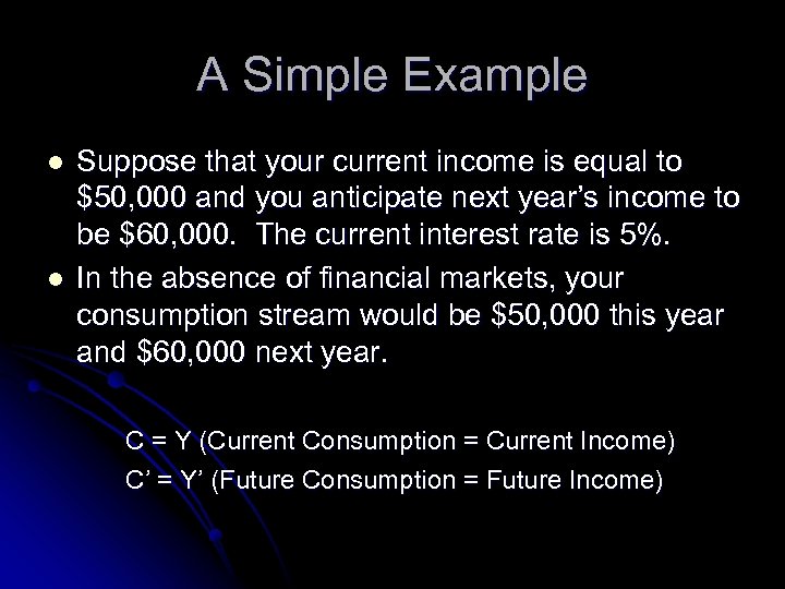A Simple Example l l Suppose that your current income is equal to $50, 000 and you anticipate next year’s income to be $60, 000. The current interest rate is 5%. In the absence of financial markets, your consumption stream would be $50, 000 this year and $60, 000 next year. C = Y (Current Consumption = Current Income) C’ = Y’ (Future Consumption = Future Income)

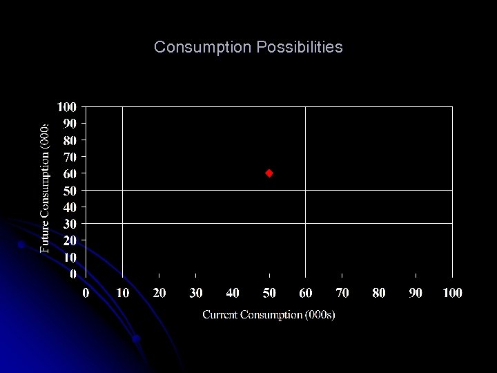Consumption Possibilities

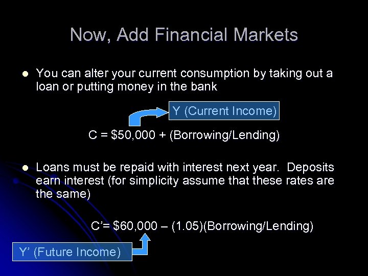Now, Add Financial Markets l You can alter your current consumption by taking out a loan or putting money in the bank Y (Current Income) C = $50, 000 + (Borrowing/Lending) l Loans must be repaid with interest next year. Deposits earn interest (for simplicity assume that these rates are the same) C’= $60, 000 – (1. 05)(Borrowing/Lending) Y’ (Future Income)

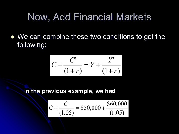Now, Add Financial Markets l We can combine these two conditions to get the following: In the previous example, we had

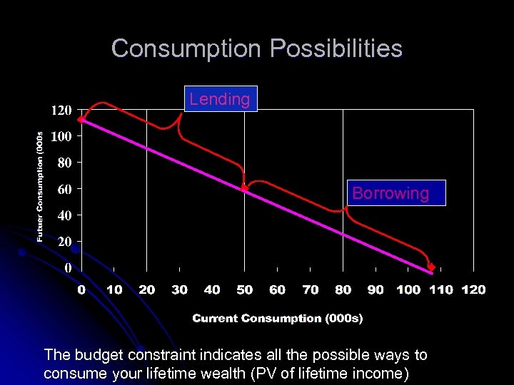Consumption Possibilities Lending Borrowing The budget constraint indicates all the possible ways to consume your lifetime wealth (PV of lifetime income)

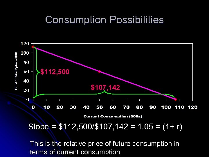Consumption Possibilities $112, 500 $107, 142 Slope = $112, 500/$107, 142 = 1. 05 = (1+ r) This is the relative price of future consumption in terms of current consumption

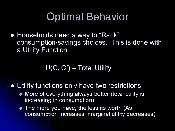Optimal Behavior l Households need a way to “Rank” consumption/savings choices. This is done with a Utility Function U(C, C’) = Total Utility functions only have two restrictions l l More of everything always better (total utility is increasing in consumption) The more you have, the less its worth (As consumption increases, marginal utility decreases)

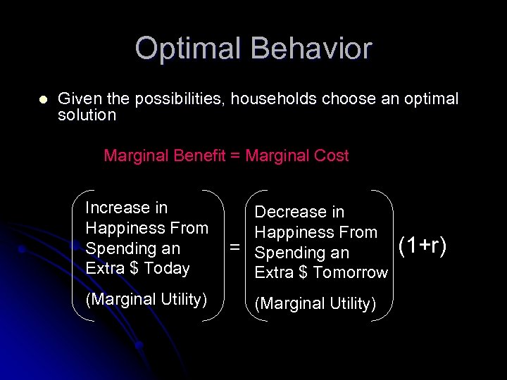Optimal Behavior l Given the possibilities, households choose an optimal solution Marginal Benefit = Marginal Cost Increase in Happiness From Spending an Extra $ Today (Marginal Utility) Decrease in Happiness From = Spending an Extra $ Tomorrow (Marginal Utility) (1+r)

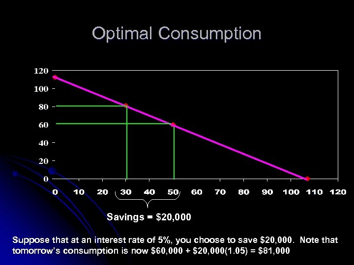Optimal Consumption Savings = $20, 000 Suppose that at an interest rate of 5%, you choose to save $20, 000. Note that tomorrow’s consumption is now $60, 000 + $20, 000(1. 05) = $81, 000

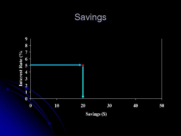Savings

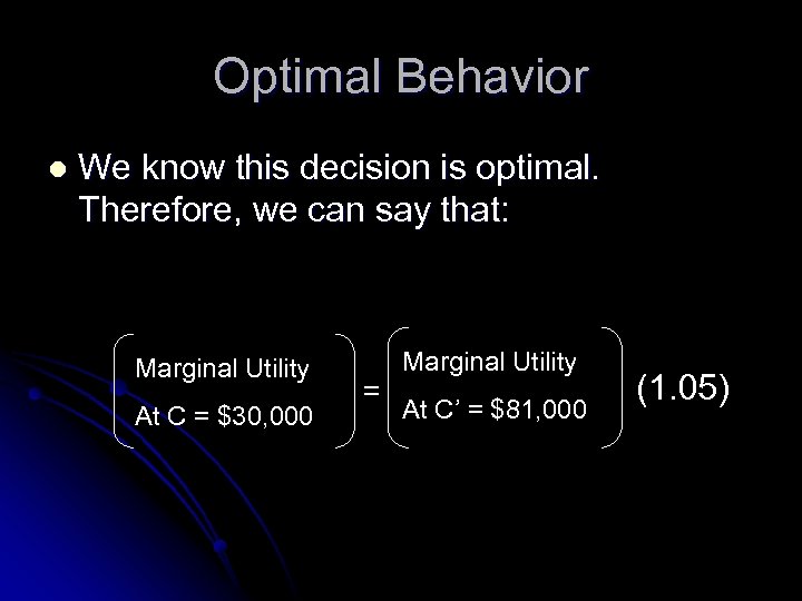Optimal Behavior l We know this decision is optimal. Therefore, we can say that: Marginal Utility At C = $30, 000 = Marginal Utility At C’ = $81, 000 (1. 05)

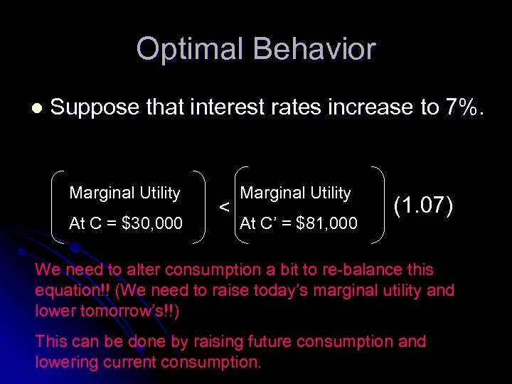Optimal Behavior l Suppose that interest rates increase to 7%. Marginal Utility At C = $30, 000 < Marginal Utility At C’ = $81, 000 (1. 07) We need to alter consumption a bit to re-balance this equation!! (We need to raise today’s marginal utility and lower tomorrow’s!!) This can be done by raising future consumption and lowering current consumption.

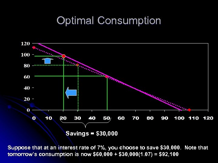Optimal Consumption Savings = $30, 000 Suppose that at an interest rate of 7%, you choose to save $30, 000. Note that tomorrow’s consumption is now $60, 000 + $30, 000(1. 07) = $92, 100

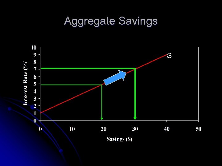Aggregate Savings S

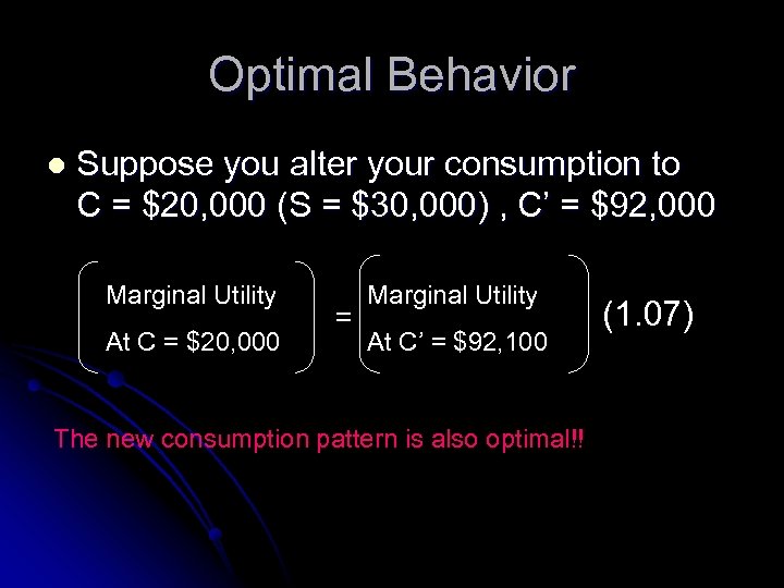Optimal Behavior l Suppose you alter your consumption to C = $20, 000 (S = $30, 000) , C’ = $92, 000 Marginal Utility At C = $20, 000 = Marginal Utility At C’ = $92, 100 The new consumption pattern is also optimal!! (1. 07)

Again, assume that the interest rate is 5%, consider two individuals Person A Current income: $10, 000 Anticipated future income: $50, 000 Wealth: $57, 619 Person B Current Income: $50, 000 Anticipated Future income: $8, 000 Wealth: $57, 619

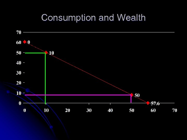Consumption and Wealth

Consumption and Wealth l l With capital markets, consumption is not determined by current income, but by wealth (present value of lifetime income) These two individuals, having the same wealth, should choose the same consumption

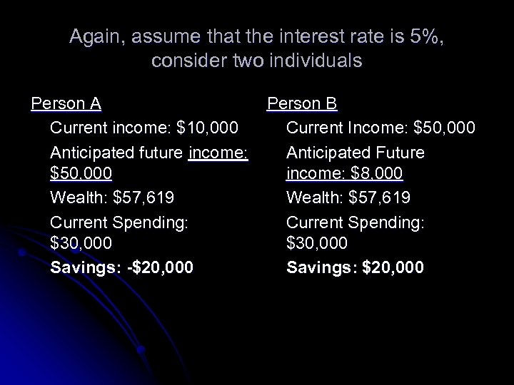Again, assume that the interest rate is 5%, consider two individuals Person A Current income: $10, 000 Anticipated future income: $50, 000 Wealth: $57, 619 Current Spending: $30, 000 Savings: -$20, 000 Person B Current Income: $50, 000 Anticipated Future income: $8, 000 Wealth: $57, 619 Current Spending: $30, 000 Savings: $20, 000

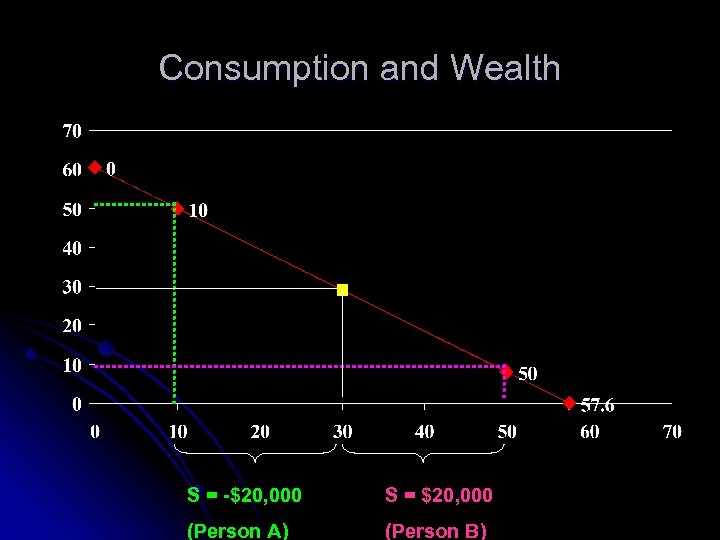Consumption and Wealth S = -$20, 000 S = $20, 000 (Person A) (Person B)

Consumption and Wealth l l l With capital markets, consumption is not determined by current income, but by wealth (present value of lifetime income) These two individuals, having the same wealth, should choose the same consumption. For a given level of wealth, savings declines with income growth

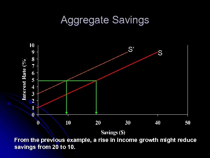Aggregate Savings S’ S From the previous example, a rise in income growth might reduce savings from 20 to 10.

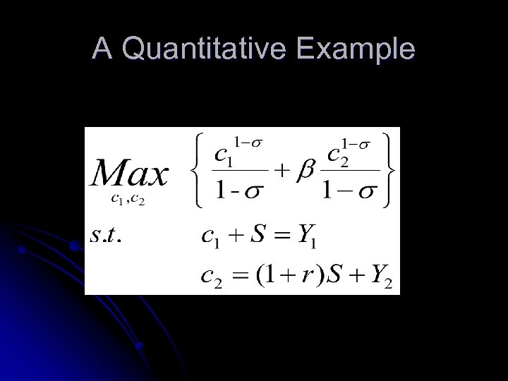A Quantitative Example

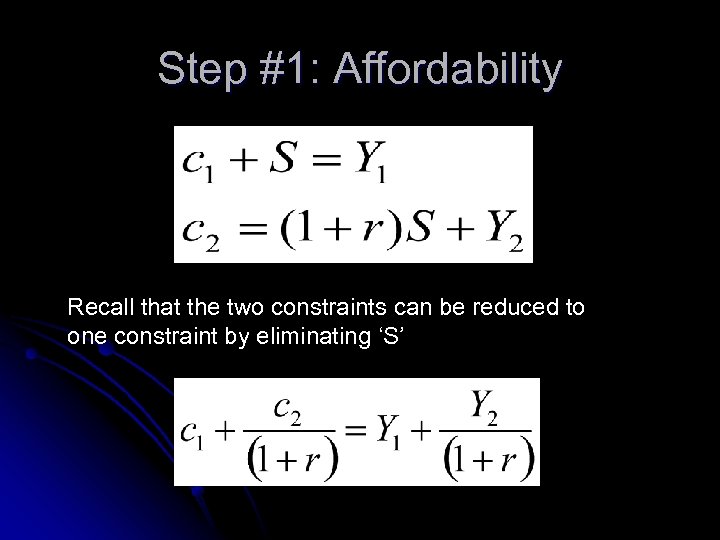Step #1: Affordability Recall that the two constraints can be reduced to one constraint by eliminating ‘S’

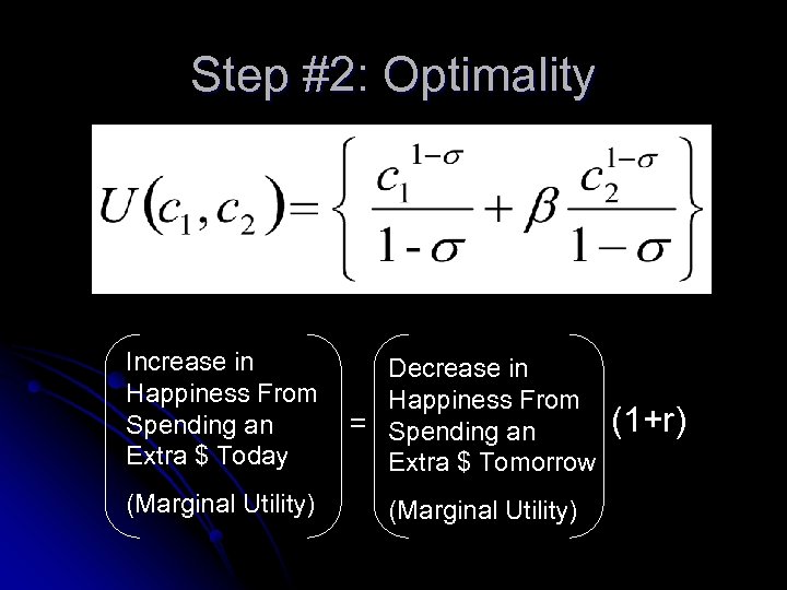Step #2: Optimality Increase in Happiness From Spending an Extra $ Today (Marginal Utility) Decrease in Happiness From = Spending an Extra $ Tomorrow (Marginal Utility) (1+r)

Step #2: Optimality Marginal Utilities are just the derivatives!! Marginal Utility Today Marginal Utility Tomorrow

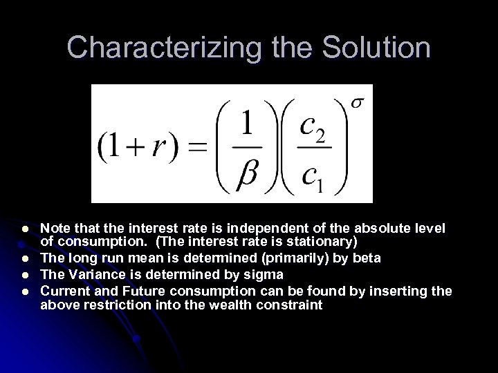Characterizing the Solution l l Note that the interest rate is independent of the absolute level of consumption. (The interest rate is stationary) The long run mean is determined (primarily) by beta The Variance is determined by sigma Current and Future consumption can be found by inserting the above restriction into the wealth constraint

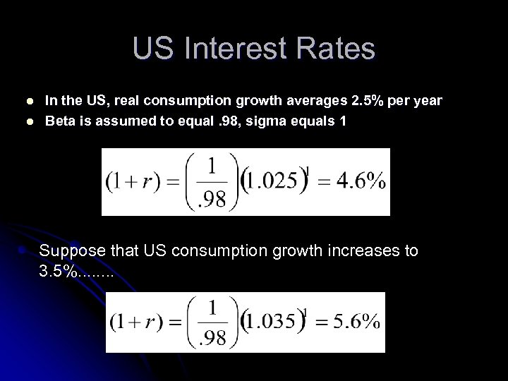US Interest Rates l l In the US, real consumption growth averages 2. 5% per year Beta is assumed to equal. 98, sigma equals 1 Suppose that US consumption growth increases to 3. 5%. . . .

Capital Investment l l Investment refers to the purchase of new capital equipment by the private sector Firms only invest in projects that add to shareholder value. Therefore, they invest in positive net present value projects. Present Value of Lifetime Profits > Cost

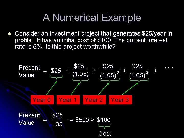A Numerical Example l Consider an investment project that generates $25/year in profits. It has an initial cost of $100. The current interest rate is 5%. Is this project worthwhile? $25 $25 Present = $25 + (1. 05) 2 + (1. 05) 3 + Value Year 0 Year 1 Present $25 Value =. 05 Year 2 Year 3 = $500 > $100 Cost . . .

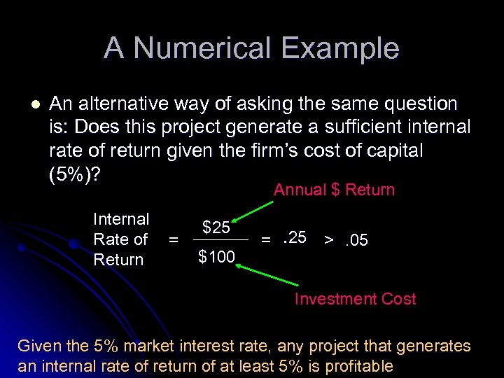A Numerical Example l An alternative way of asking the same question is: Does this project generate a sufficient internal rate of return given the firm’s cost of capital (5%)? Annual $ Return Internal Rate of Return = $25 $100 = . 25 >. 05 Investment Cost Given the 5% market interest rate, any project that generates an internal rate of return of at least 5% is profitable

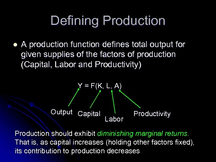Defining Production l A production function defines total output for given supplies of the factors of production (Capital, Labor and Productivity) Y = F(K, L, A) Output Capital Labor Productivity Production should exhibit diminishing marginal returns. That is, as capital increases (holding other factors fixed), its contribution to production decreases

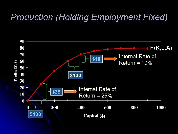Production (Holding Employment Fixed) F(K, L, A) $100 $25 $100 Internal Rate of Return = 25% Internal Rate of Return = 10%

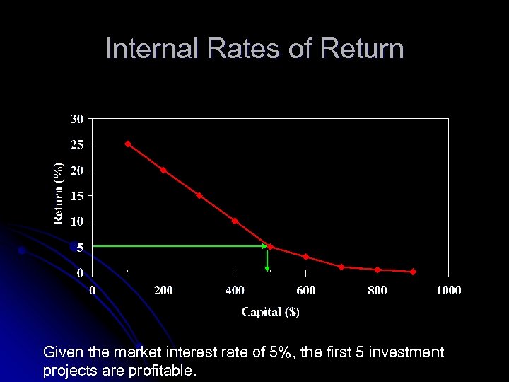Internal Rates of Return Given the market interest rate of 5%, the first 5 investment projects are profitable.

Investment Demand l l l It is assumed that labor and capital are compliments. That is, when employment rises, the productivity of capital increases as well. Therefore, as a rise in employment should increase the demand for capital and, hence, the demand for loans Further, any technological improvement should also raise the demand for investment

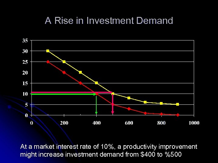A Rise in Investment Demand At a market interest rate of 10%, a productivity improvement might increase investment demand from $400 to %500

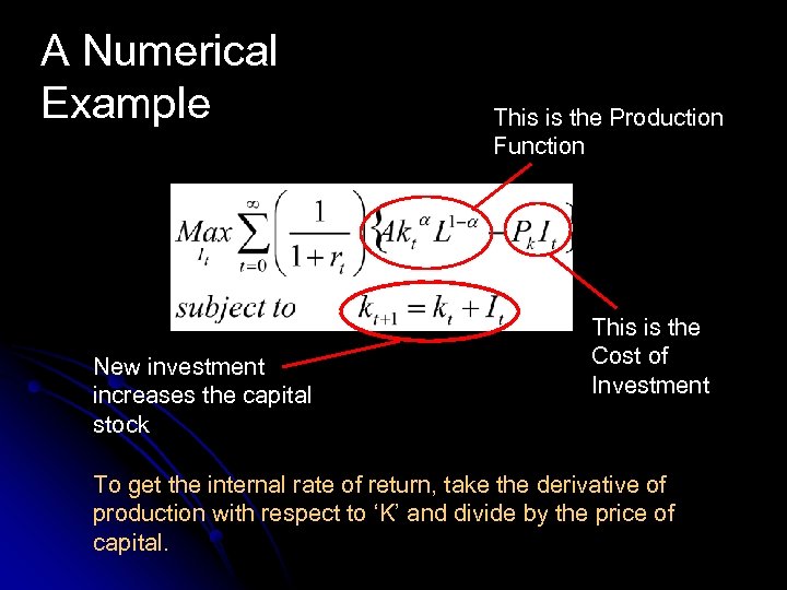A Numerical Example New investment increases the capital stock This is the Production Function This is the Cost of Investment To get the internal rate of return, take the derivative of production with respect to ‘K’ and divide by the price of capital.

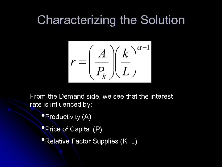Characterizing the Solution From the Demand side, we see that the interest rate is influenced by: • Productivity (A) • Price of Capital (P) • Relative Factor Supplies (K, L)

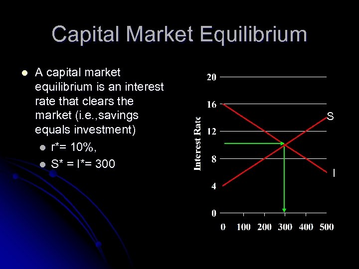Capital Market Equilibrium l A capital market equilibrium is an interest rate that clears the market (i. e. , savings equals investment) l r*= 10%, l S* = I*= 300 S I

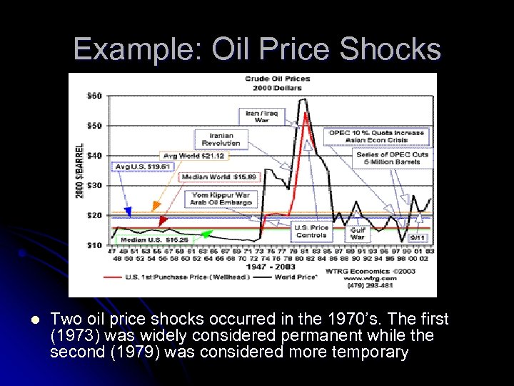Example: Oil Price Shocks l Two oil price shocks occurred in the 1970’s. The first (1973) was widely considered permanent while the second (1979) was considered more temporary

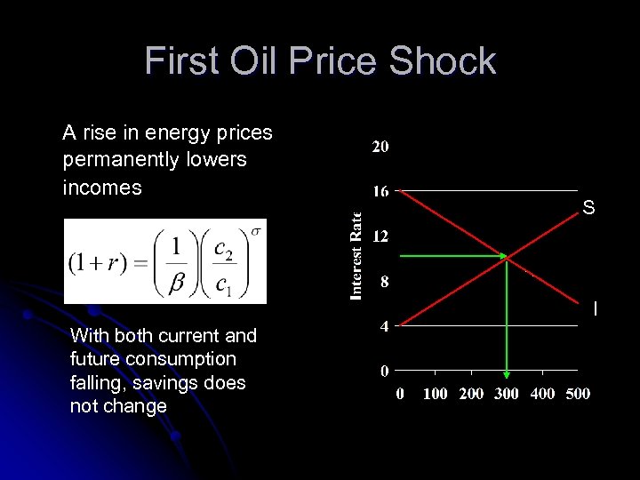First Oil Price Shock A rise in energy prices permanently lowers incomes S I With both current and future consumption falling, savings does not change

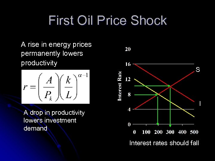First Oil Price Shock A rise in energy prices permanently lowers productivity S I A drop in productivity lowers investment demand Interest rates should fall

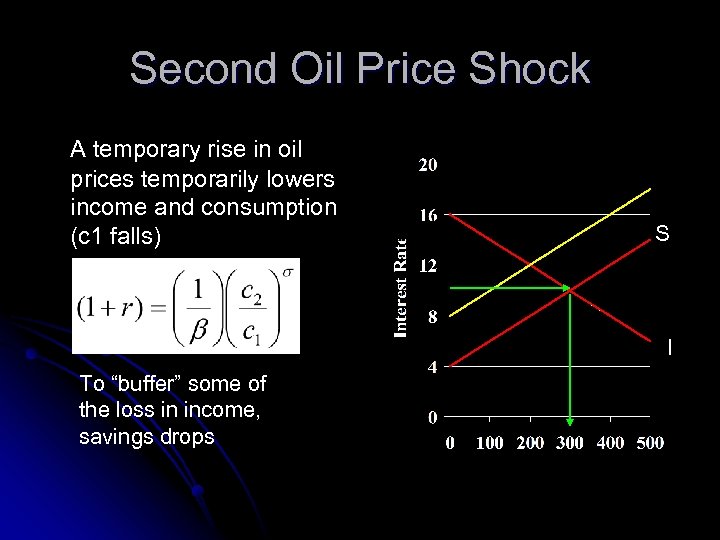Second Oil Price Shock A temporary rise in oil prices temporarily lowers income and consumption (c 1 falls) S I To “buffer” some of the loss in income, savings drops

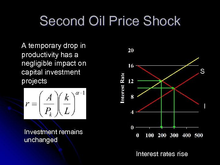Second Oil Price Shock A temporary drop in productivity has a negligible impact on capital investment projects S I Investment remains unchanged Interest rates rise

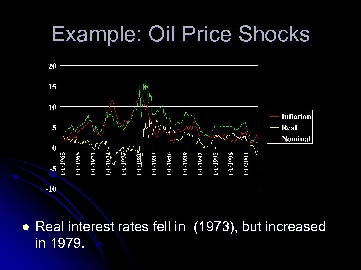Example: Oil Price Shocks l Real interest rates fell in (1973), but increased in 1979.

Government Deficits and Interest Rates l Last year, the government borrowed roughly $450 billion from financial markets. Should this have an impact on real interest rates?

Nominal Interest Rates & Inflation l i = r + Inflation? l Wealth effects (Higher inflation lowers the purchasing power of lifetime wealth) l The Darby effect (The government taxes nominal income) l Expected vs. Actual inflation

Nominal Interest Rates & the Fed l The Federal Reserve has two potentially offsetting effects on the nominal interest rate: l Liquidity Effect l Anticipated Inflation effect

Forecasting Nominal Interest Rate l Any Interest rate equation could potentially have any of the following variables: l Income Growth l Proxies for productivity l Relative price of capital l Government Deficits l Inflation Rates l Monetary Policy Variables

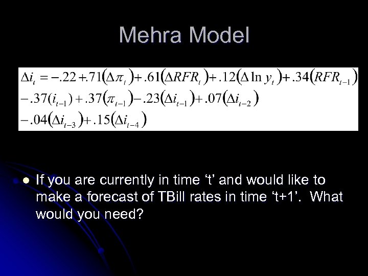Mehra Model l If you are currently in time ‘t’ and would like to make a forecast of TBill rates in time ‘t+1’. What would you need?

Mehra Model l To Forecast the TBill rate, you need: l. A Forecast for price (to calculate the inflation rate) l A Forecast of Federal Reserve Policy l A Forecast of GDP (to calculate income growth) l Past history of TBill Rates and Inflation