87be6ec4e5b363edde96b61ef8598702.ppt
- Количество слайдов: 8
FNR 407 Forest Economics William L. (Bill) Hoover Professor of Forestry 494 -3580 743 -4120 whoover@purdue. edu

Economics y pp l Su Price (P) – Market – Other, e. g. ? (S ) • Allocation of scarce resources to unlimited wants De ma nd (D ) Quantity (Q)
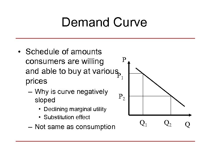
Demand Curve • Schedule of amounts P consumers are willing and able to buy at various. P 1 prices – Why is curve negatively sloped • Declining marginal utility • Substitution effect – Not same as consumption P 2 Q 1 Q 2 Q
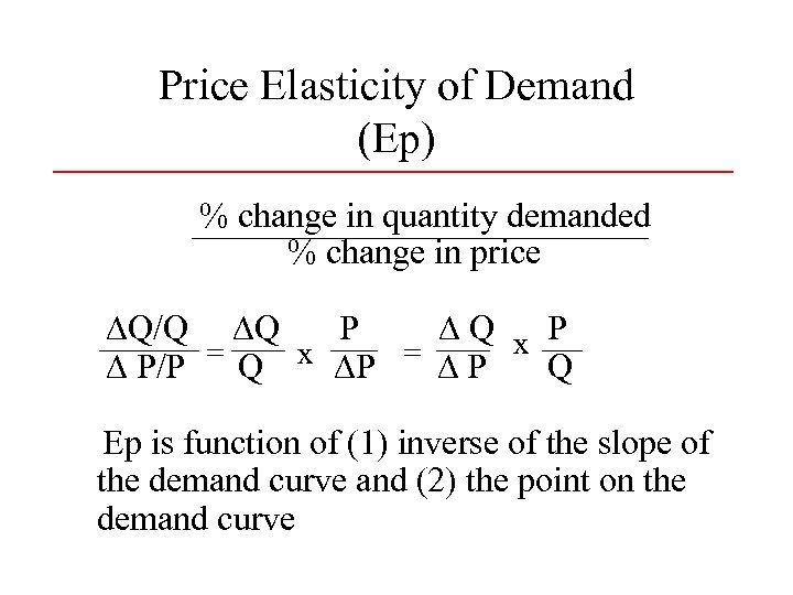
Price Elasticity of Demand (Ep) % change in quantity demanded % change in price ∆Q/Q ∆Q P ∆Q x P ∆ P/P = Q x ∆P = ∆ P Q Ep is function of (1) inverse of the slope of the demand curve and (2) the point on the demand curve
Relationship of Ep to Total Revenue • When Ep > |1|, decreasing price increases total revenue (the elastic range of the demand curve) • When Ep = 1, total revenue is maximized • When Ep < |1|, decreasing price decreases total revenue (the inelastic range of the demand curve)
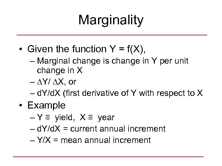
Marginality • Given the function Y = f(X), – Marginal change is change in Y per unit change in X – ∆Y/ ∆X, or – d. Y/d. X (first derivative of Y with respect to X • Example – Y ≡ yield, X ≡ year – d. Y/d. X = current annual increment – Y/X = mean annual increment
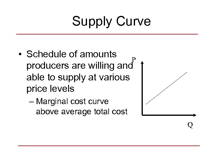
Supply Curve • Schedule of amounts P producers are willing and able to supply at various price levels – Marginal cost curve above average total cost Q
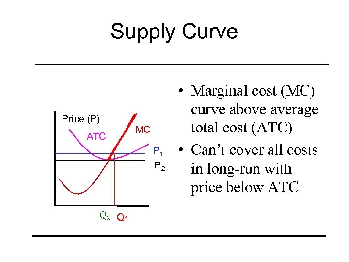
Supply Curve Price (P) ATC MC P 1 P 2 Q 1 • Marginal cost (MC) curve above average total cost (ATC) • Can’t cover all costs in long-run with price below ATC
87be6ec4e5b363edde96b61ef8598702.ppt