7c44680d7710ed6871d70d6085f96975.ppt
- Количество слайдов: 93
FIXED INCOME SECURITIES LECTURE 6 BOND RISK
债券风险 (1)利率风险; (2)违约风险(信用风险); (3)通货膨胀风险; (4)提前偿还风险; (5)汇率风险; (6)流动性风险。
Default Risk (1) • Default Risk: Uncertainty that the realized return will deviate from the expected return because the issuer will fail to meet the contractual obligations specified in the indenture. • The major concern is failure to meet interest and principal payments.
Default Risk: Points (2) • Most investors do not directly access a bond’s default risk, but instead use the quality ratings provided by Moody’s, S&P, and Fetch to evaluate the degree of risk. – AAA, A, BBB, ……, C, …… • Default Rates: –. 12% per year for all bonds since WWII. – 1980 s: 3. 27% per year on junk bonds. – 1990 -1991: 9% on junk bonds
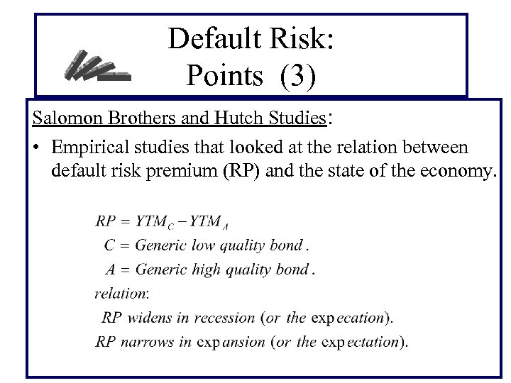
Default Risk: Points (3) Salomon Brothers and Hutch Studies: • Empirical studies that looked at the relation between default risk premium (RP) and the state of the economy.
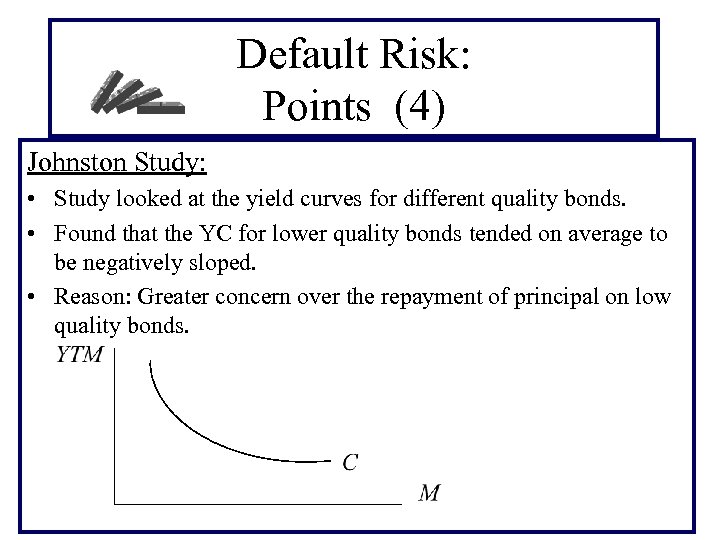
Default Risk: Points (4) Johnston Study: • Study looked at the yield curves for different quality bonds. • Found that the YC for lower quality bonds tended on average to be negatively sloped. • Reason: Greater concern over the repayment of principal on low quality bonds.
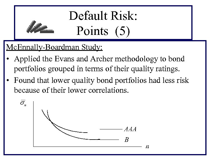
Default Risk: Points (5) Mc. Ennally-Boardman Study: • Applied the Evans and Archer methodology to bond portfolios grouped in terms of their quality ratings. • Found that lower quality bond portfolios had less risk because of their lower correlations.
Call Risk (1) • Call Risk: Uncertainty that the realized return will deviate from the expected return because the issuer calls the bond, forcing the investor to reinvest in a market with lower rates. • Note: When a bond is called the holder receives the call price (CP). Since the CP usually exceeds the principal, the return the investor receives over the call period is often greater than the initial YTM. The investor, though, usually has to reinvest in a market with lower rates which often causes his return for the investment period to be less than the initial YTM.
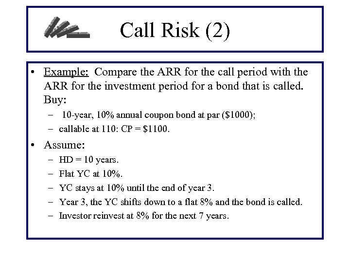
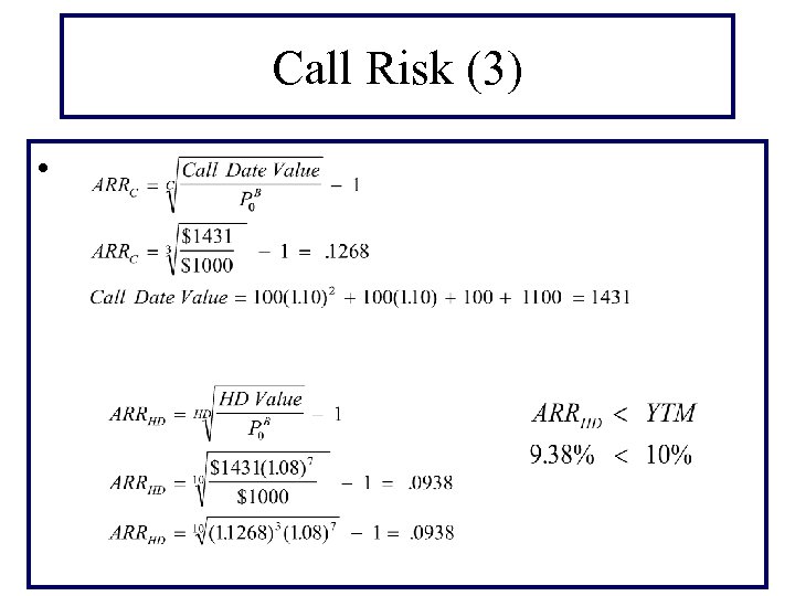
Call Risk (2) • Example: Compare the ARR for the call period with the ARR for the investment period for a bond that is called. Buy: – 10 -year, 10% annual coupon bond at par ($1000); – callable at 110: CP = $1100. • Assume: – – – HD = 10 years. Flat YC at 10%. YC stays at 10% until the end of year 3. Year 3, the YC shifts down to a flat 8% and the bond is called. Investor reinvest at 8% for the next 7 years.
Call Risk (3) •
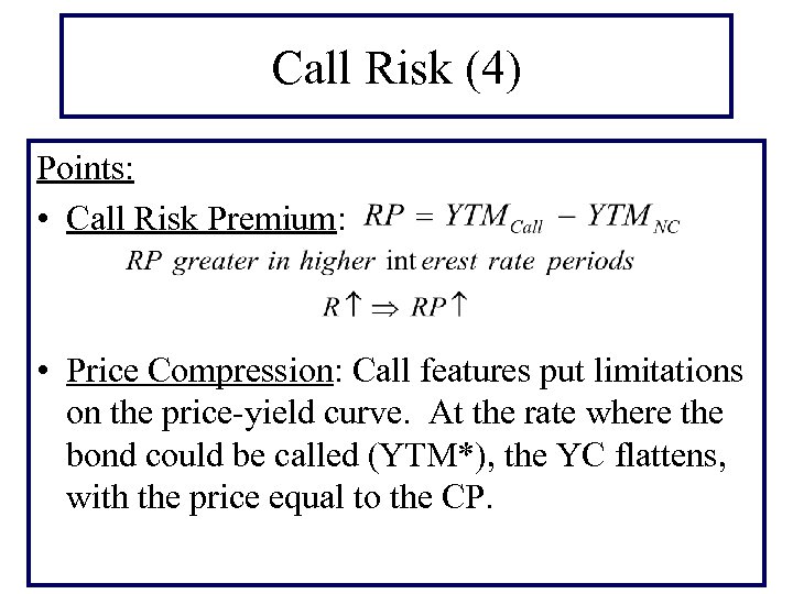
Call Risk (4) Points: • Call Risk Premium: • Price Compression: Call features put limitations on the price-yield curve. At the rate where the bond could be called (YTM*), the YC flattens, with the price equal to the CP.
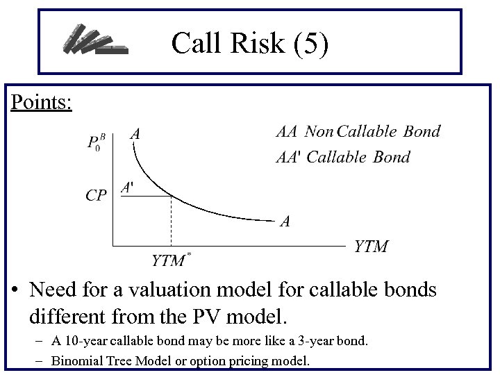
Call Risk (5) Points: • Need for a valuation model for callable bonds different from the PV model. – A 10 -year callable bond may be more like a 3 -year bond. – Binomial Tree Model or option pricing model.
债券利率风险 • 包括: 价格(市场)风险; 再投 资风险 • 所有债券价格都受利率变化 的影响 • 对于高等级债券利率风险更 重要
债券价值和收益率的关系 • 假定未来现金流的数额和时间都是确定 的,其风险通过贴现率来调整 • 例子: – ATT 6 s 09 – 面值 = $1, 000; 到期日: Oct. 15, 2009 – 年利息=(6% of $1, 000)/2=$30 – 支付日: April 15, October 15
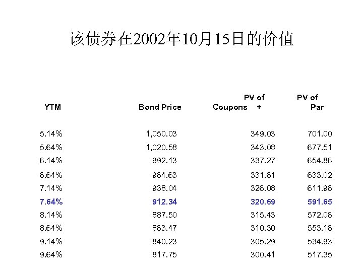
该债券在 2002年 10月15日的价值 PV of Coupons + PV of Par YTM Bond Price 5. 14% 1, 050. 03 349. 03 701. 00 5. 64% 1, 020. 58 343. 08 677. 51 6. 14% 992. 13 337. 27 654. 86 6. 64% 964. 63 331. 61 633. 02 7. 14% 938. 04 326. 08 611. 96 7. 64% 912. 34 320. 69 591. 65 8. 14% 887. 50 315. 43 572. 06 8. 64% 863. 47 310. 30 553. 16 9. 14% 840. 23 305. 29 534. 93 9. 64% 817. 75 300. 41 517. 35
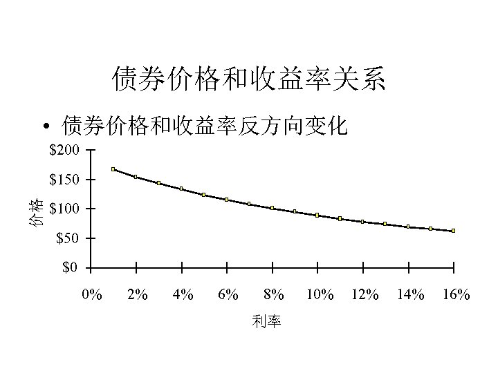
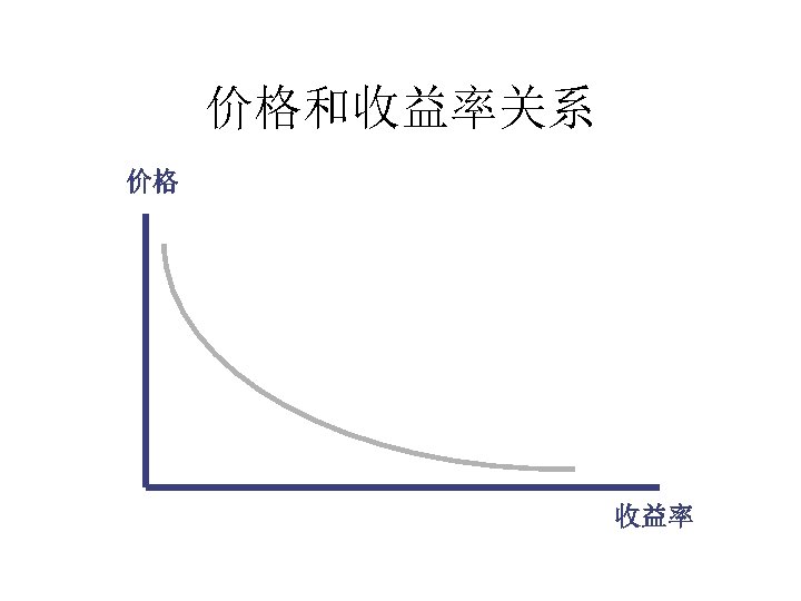
债券价格和收益率关系 • 债券价格和收益率反方向变化 $200 价格 $150 $100 $50 $0 0% 2% 4% 6% 8% 利率 10% 12% 14% 16%
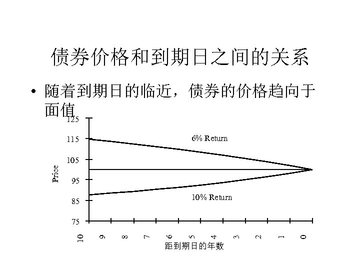
债券价格和到期日之间的关系 • 随着到期日的临近,债券的价格趋向于 面值 125 6% Return 115 95 10% Return 85 距到期日的年数 0 1 2 3 4 5 6 7 8 9 75 10 Price 105
债券价格波动性的特点 1、价格的利率敏感性与债券的票面利率具有反 向关系。其他因素相同时,低票面利率债券比 高票面利率债券价格的利率敏感性更强。 2、价格的利率敏感性与债券的到期时间长短具 有正向关系。其他因素相同时,长期债券比短 期债券价格的利率敏感性更强。 3、随着到期时间的增长,价格的利率敏感性增 加,但是增加得越来越慢。
债券价格波动性的特点(续) 4、收益率上升导致价格下跌的幅度比 等规模的收益率降低带来的价格上涨的 幅度小,这被称为价格波动的不对称性。 5、价格的利率敏感性与债券的初始收益 率水平具有反向关系。其他因素相同时, 债券的初始收益率较低时,价格的利率 敏感性更强。
Bond Pricing Relationships • Inverse relationship between price and yield • An increase in a bond’s yield to maturity results in a smaller price decline than the gain associated with a decrease in yield • Long-term bonds tend to be more price sensitive than short-term bonds
Bond Pricing Relationships (cont. ) • As maturity increases, price sensitivity increases at a decreasing rate • Price sensitivity is inversely related to a bond’s coupon rate • Price sensitivity is inversely related to the yield to maturity at which the bond is selling
价格和收益率关系 价格 收益率
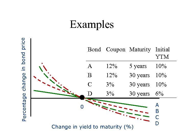
Bond Coupon Maturity Initial YTM A B C D 12% 3% 3% 5 years 30 years 0 Percentage change in bond price Examples Change in yield to maturity (%) 10% 10% 6% A B C D
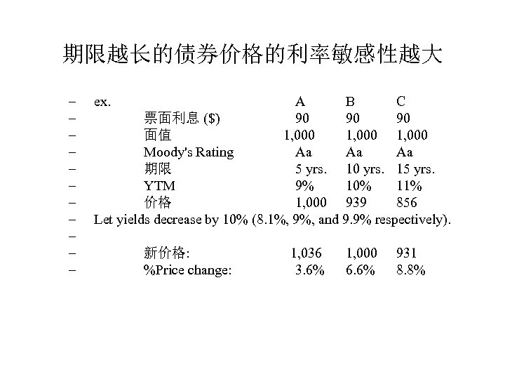
期限越长的债券价格的利率敏感性越大 – – – ex. A B C 票面利息 ($) 90 90 90 面值 1, 000 Moody's Rating Aa Aa Aa 期限 5 yrs. 10 yrs. 15 yrs. YTM 9% 10% 11% 价格 1, 000 939 856 Let yields decrease by 10% (8. 1%, 9%, and 9. 9% respectively). 新价格: 1, 036 1, 000 931 %Price change: 3. 6% 6. 6% 8. 8%
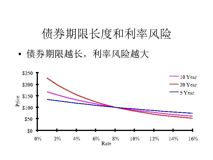
债券期限长度和利率风险 • 债券期限越长,利率风险越大 $250 10 Year 20 Year 5 Year Price $200 $150 $100 $50 $0 0% 2% 4% 6% Rate 8% 10% 12% 14% 16%
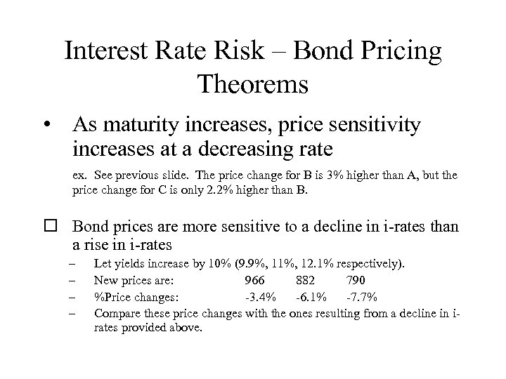
Interest Rate Risk – Bond Pricing Theorems • As maturity increases, price sensitivity increases at a decreasing rate ex. See previous slide. The price change for B is 3% higher than A, but the price change for C is only 2. 2% higher than B. o Bond prices are more sensitive to a decline in i-rates than a rise in i-rates – – Let yields increase by 10% (9. 9%, 11%, 12. 1% respectively). New prices are: 966 882 790 %Price changes: -3. 4% -6. 1% -7. 7% Compare these price changes with the ones resulting from a decline in irates provided above.
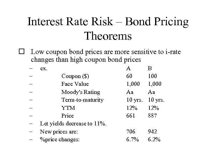
Interest Rate Risk – Bond Pricing Theorems o Low coupon bond prices are more sensitive to i-rate changes than high coupon bond prices – – – – – ex. Coupon ($) Face Value Moody's Rating Term-to-maturity YTM Price Let yields decrease to 11%. New prices are: %price changes: A 60 1, 000 Aa 10 yrs. 12% 661 B 100 1, 000 Aa 10 yrs. 12% 887 706 6. 7% 942 6. 2%
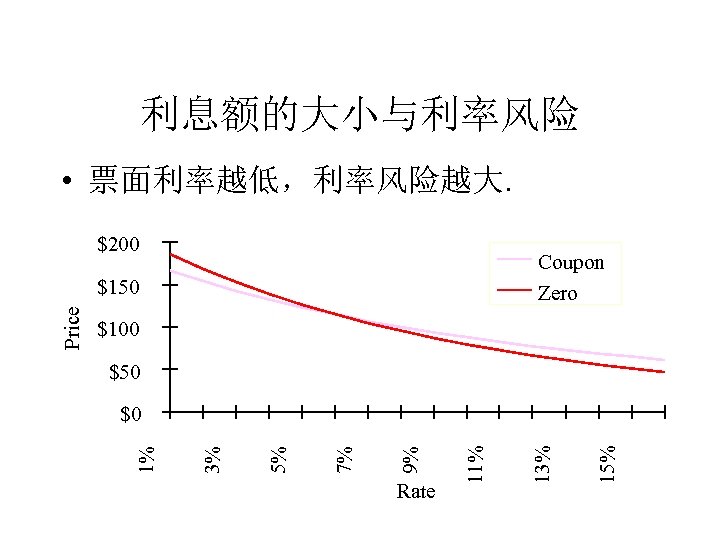
利息额的大小与利率风险 • 票面利率越低,利率风险越大. $200 Coupon Zero $100 $50 15% 13% Rate 11% 9% 7% 5% 3% $0 1% Price $150
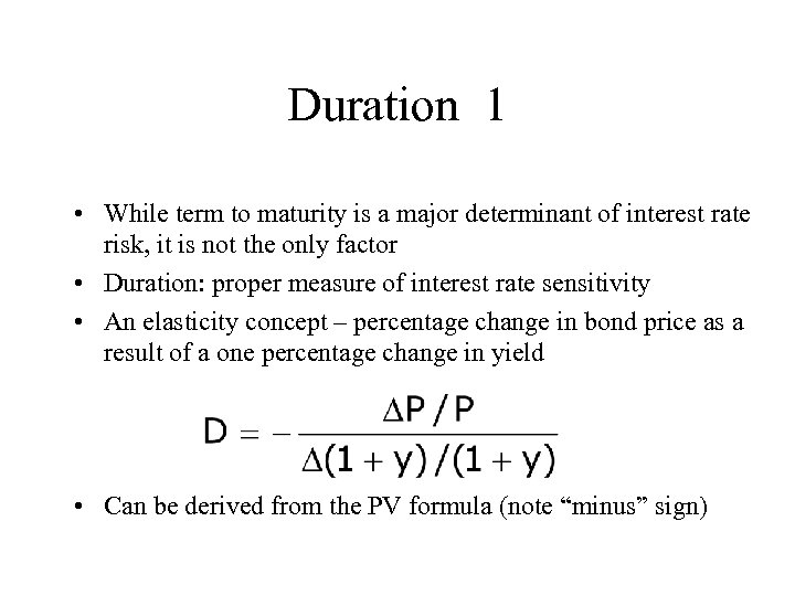
Duration 1 • While term to maturity is a major determinant of interest rate risk, it is not the only factor • Duration: proper measure of interest rate sensitivity • An elasticity concept – percentage change in bond price as a result of a one percentage change in yield • Can be derived from the PV formula (note “minus” sign)
Duration 2 • A measure of the effective maturity of a bond • The weighted average of the times until each payment is received, with the weights proportional to the present value of the payment
Why is duration important? • Measures the interest rate risk of a bond • Allows comparison across bonds that differ in coupon rate, yield and maturity • Also a measure of the effective maturity of a bond (weighted average maturity of a bond’s cash flows) • An essential concept in bond portfolio management, particularly in immunization strategies (protecting bond portfolios from interest rate risk)
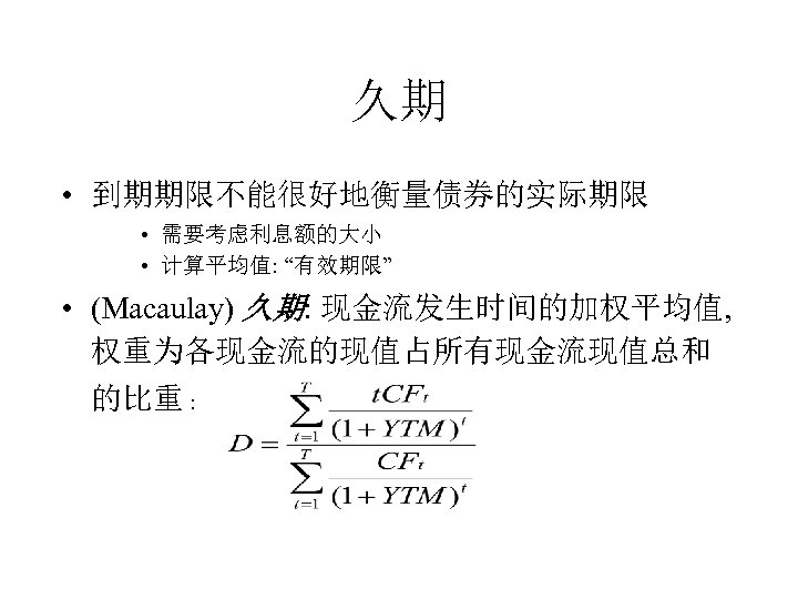
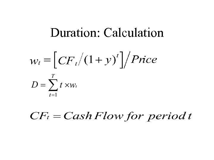
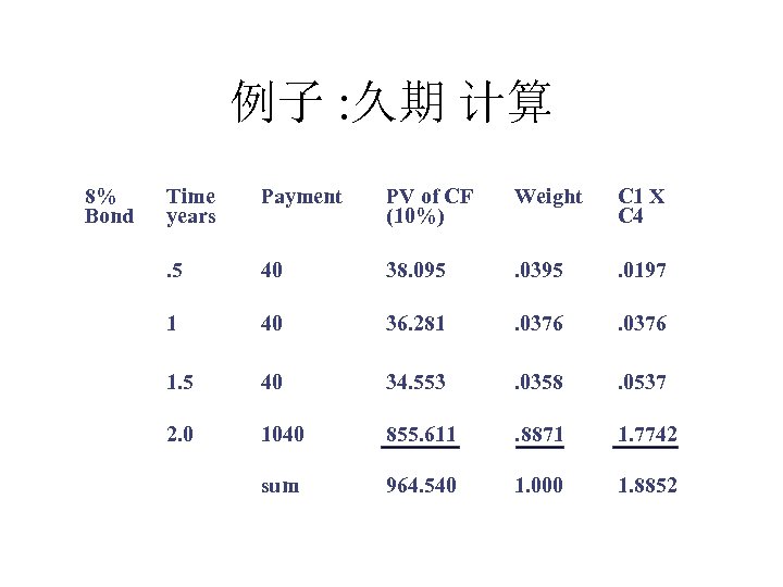
久期 • 到期期限不能很好地衡量债券的实际期限 • 需要考虑利息额的大小 • 计算平均值: “有效期限” • (Macaulay) 久期: 现金流发生时间的加权平均值, 权重为各现金流的现值占所有现金流现值总和 的比重 :
Duration: Calculation
Duration Calculation
例子 : 久期 计算 8% Bond Time years Payment PV of CF (10%) Weight C 1 X C 4 . 5 40 38. 095 . 0395 . 0197 1 40 36. 281 . 0376 1. 5 40 34. 553 . 0358 . 0537 2. 0 1040 855. 611 . 8871 1. 7742 sum 964. 540 1. 000 1. 8852
开发银行债券的久期 – 发行人 开发银行 – 面值 100 – 票面利率 8% – 期限 10 年 • 假设该债券市场价格为 114. 72元,要求的利率为 6%。 存续期可计算如下:
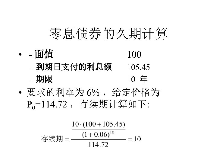
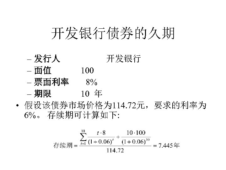
零息债券的久期计算 • - 面值 100 – 到期日支付的利息额 – 期限 105. 45 10 年 • 要求的利率为 6% ,给定价格为 P 0=114. 72 ,存续期计算如下:
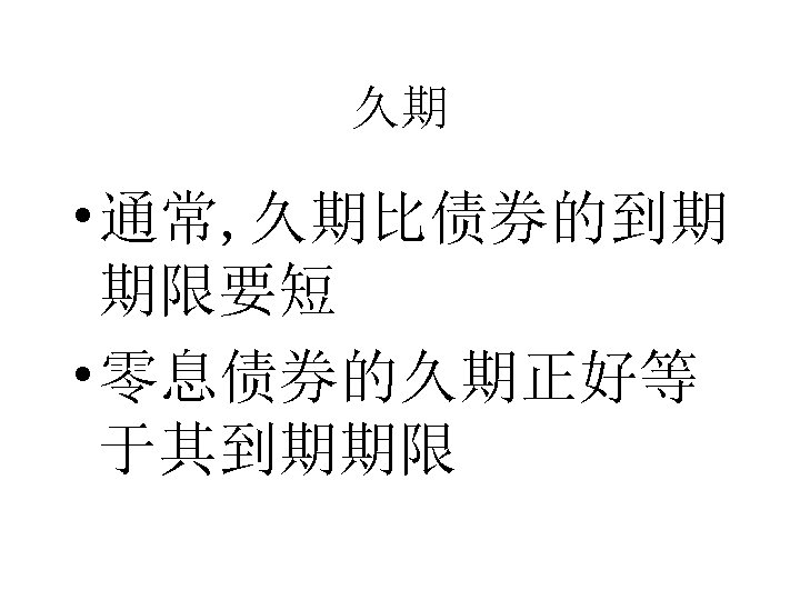
久期 • 通常, 久期比债券的到期 期限要短 • 零息债券的久期正好等 于其到期期限
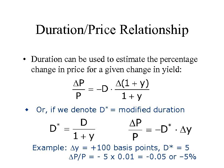
Duration/Price Relationship • Duration can be used to estimate the percentage change in price for a given change in yield: w Or, if we denote D* = modified duration Example: y = +100 basis points, D* = 5 P/P = - 5 x 0. 01 = -0. 05 or – 5%

Duration/Price Relationship • Duration can be used to estimate the percentage change in price for a given change in yield: w Or, if we denote D* = modified duration Example: y = +100 basis points, D* = 5 P/P = - 5 x 0. 01 = -0. 05 or – 5%
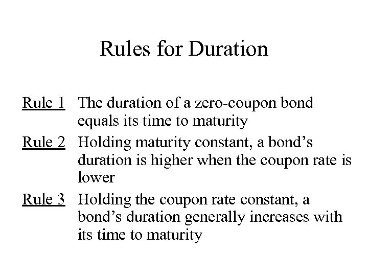
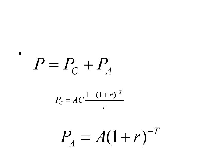
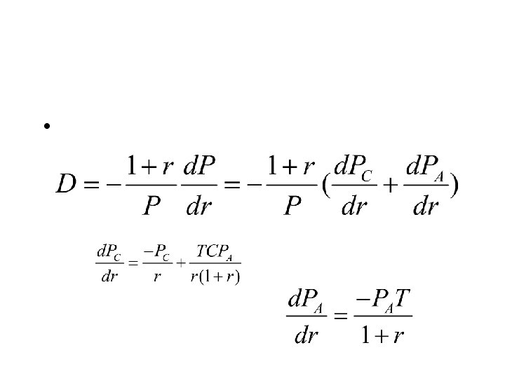
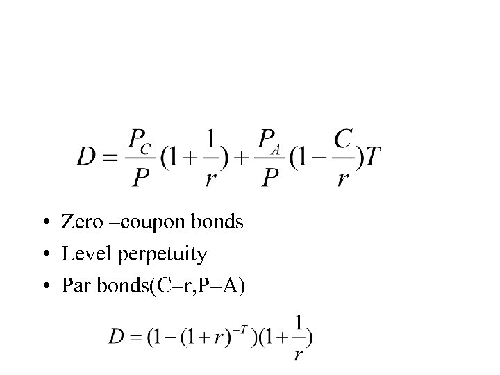
Rules for Duration Rule 1 The duration of a zero-coupon bond equals its time to maturity Rule 2 Holding maturity constant, a bond’s duration is higher when the coupon rate is lower Rule 3 Holding the coupon rate constant, a bond’s duration generally increases with its time to maturity
•
•
• Zero –coupon bonds • Level perpetuity • Par bonds(C=r, P=A)
Duration of Annuity (Mortgage)
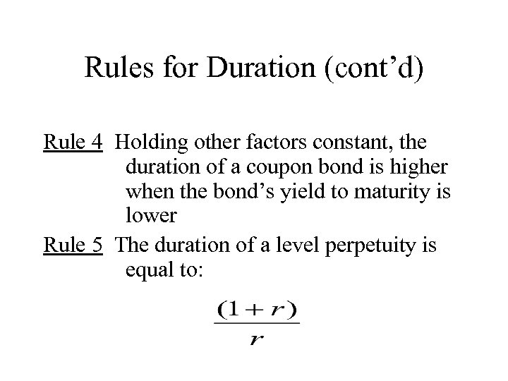
Rules for Duration (cont’d) Rule 4 Holding other factors constant, the duration of a coupon bond is higher when the bond’s yield to maturity is lower Rule 5 The duration of a level perpetuity is equal to:
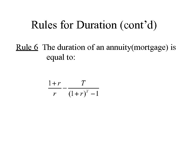
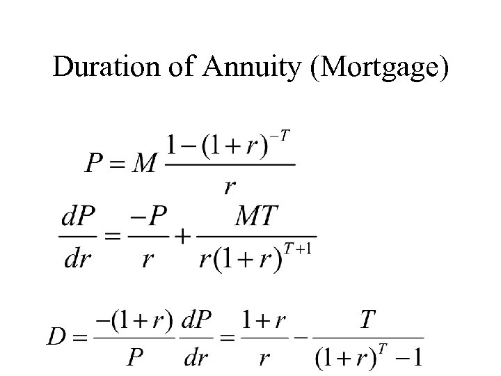
Rules for Duration (cont’d) Rule 6 The duration of an annuity(mortgage) is equal to:
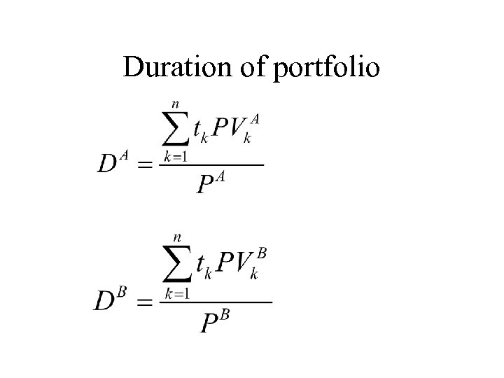
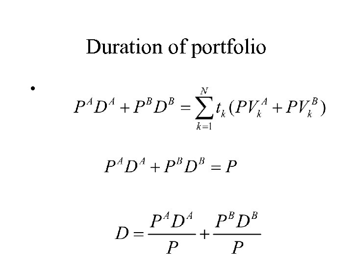
Duration of portfolio • The duration of portfolio is a weighted sum of the duration of the individual bonds— with weighting coefficients proportional to individual bond prices.
Duration of portfolio
Duration of portfolio •
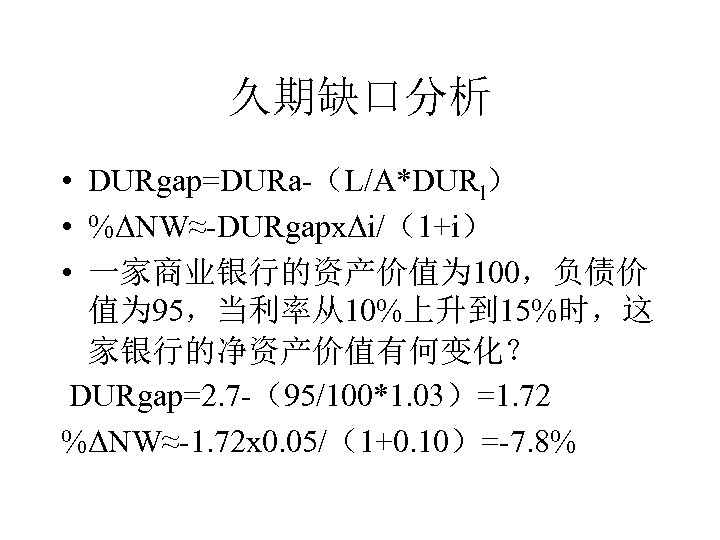
久期缺口分析 • DURgap=DURa-(L/A*DURl) • %ΔNW≈-DURgapⅹΔi/(1+i) • 一家商业银行的资产价值为 100,负债价 值为 95,当利率从10%上升到 15%时,这 家银行的净资产价值有何变化? DURgap=2. 7 -(95/100*1. 03)=1. 72 %ΔNW≈-1. 72ⅹ 0. 05/(1+0. 10)=-7. 8%
久期和凸性 Price Pricing Error from convexity Duration
Taylor expansion
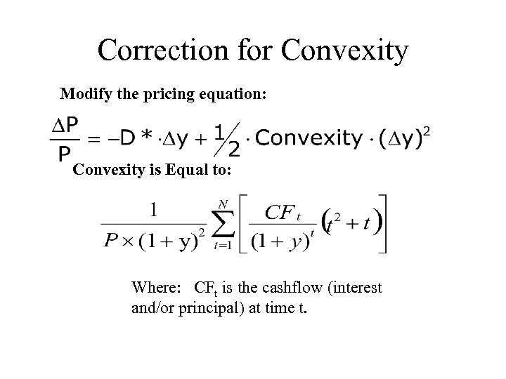
Correction for Convexity Modify the pricing equation: Convexity is Equal to: Where: CFt is the cashflow (interest and/or principal) at time t.
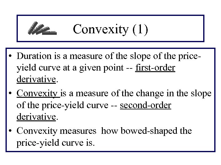
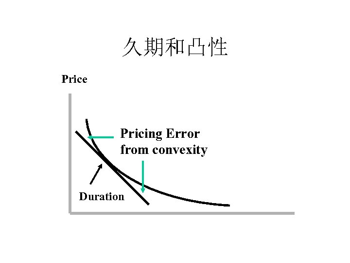
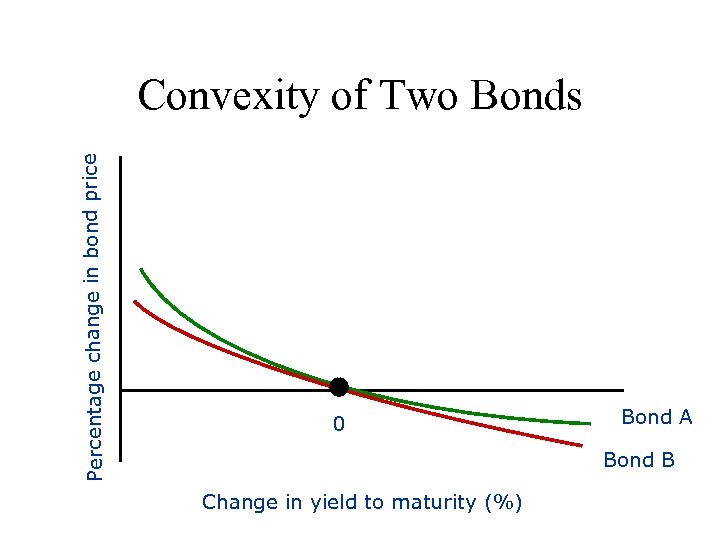
Convexity (1) • Duration is a measure of the slope of the priceyield curve at a given point -- first-order derivative. • Convexity is a measure of the change in the slope of the price-yield curve -- second-order derivative. • Convexity measures how bowed-shaped the price-yield curve is.
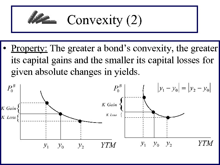
Convexity (2) • Property: The greater a bond’s convexity, the greater its capital gains and the smaller its capital losses for given absolute changes in yields.
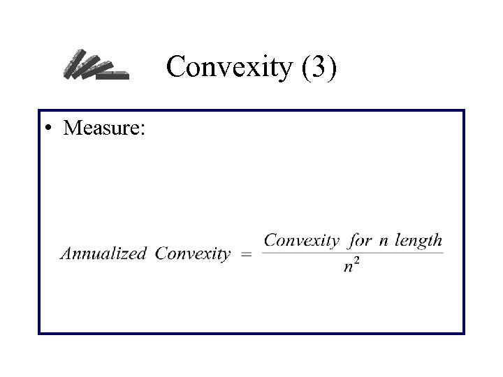
Convexity (3) • Measure:
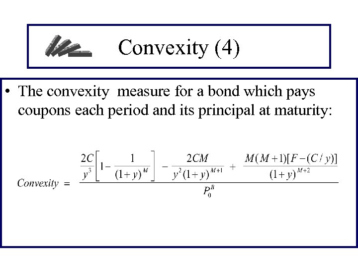
Convexity (4) • The convexity measure for a bond which pays coupons each period and its principal at maturity:
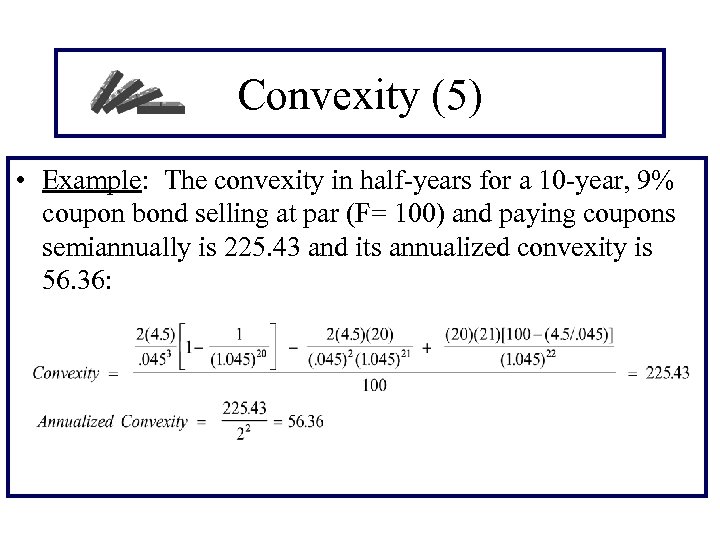
Convexity (5) • Example: The convexity in half-years for a 10 -year, 9% coupon bond selling at par (F= 100) and paying coupons semiannually is 225. 43 and its annualized convexity is 56. 36:
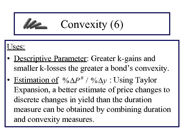
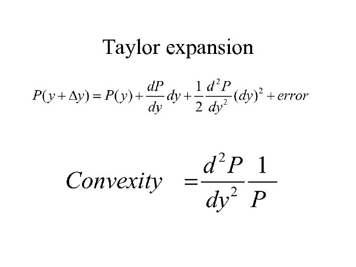
Convexity (6) Uses: • Descriptive Parameter: Greater k-gains and smaller k-losses the greater a bond’s convexity. • Estimation of : Using Taylor Expansion, a better estimate of price changes to discrete changes in yield than the duration measure can be obtained by combining duration and convexity measures.
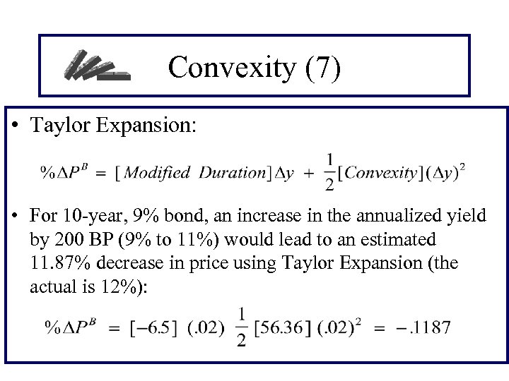
Convexity (7) • Taylor Expansion: • For 10 -year, 9% bond, an increase in the annualized yield by 200 BP (9% to 11%) would lead to an estimated 11. 87% decrease in price using Taylor Expansion (the actual is 12%):
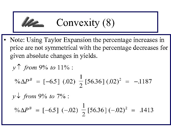
Convexity (8) • Note: Using Taylor Expansion the percentage increases in price are not symmetrical with the percentage decreases for given absolute changes in yields.
Convexity example 8% Bond Time (half year) 1 Payment PV of CF (10%) Weight (t 2+t) x C 4 40 38. 095 . 0395 . 0790 2 40 36. 281 . 0376 . 2257 3 40 34. 553 . 0358 . 4299 4 1040 855. 611 . 8871 17. 7413 sum 964. 540 1. 000 18. 4759
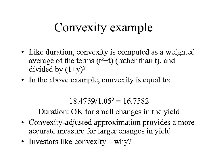
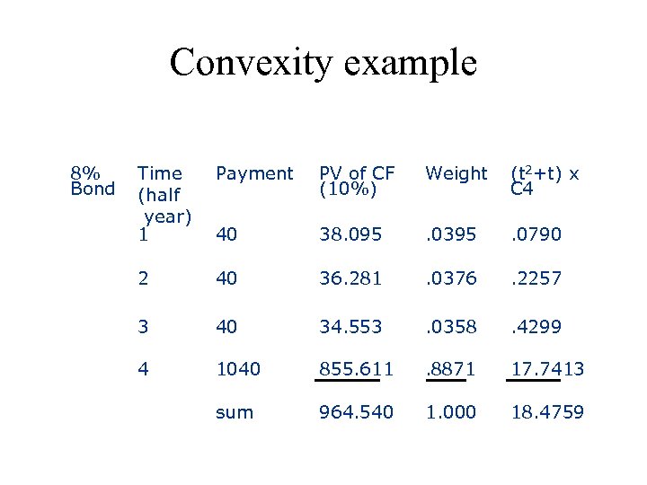
Convexity example • Like duration, convexity is computed as a weighted average of the terms (t 2+t) (rather than t), and divided by (1+y)2 • In the above example, convexity is equal to: 18. 4759/1. 052 = 16. 7582 Duration: OK for small changes in the yield • Convexity-adjusted approximation provides a more accurate measure for larger changes in yield • Investors like convexity – why?
0 Percentage change in bond price Convexity of Two Bonds Bond A Bond B Change in yield to maturity (%)
久期和凸性假定 • Derivation and application of duration and convexity assumes: – Term structure is flat – Shifts are parallel – Bonds have no imbedded options
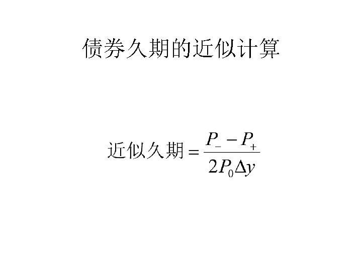
债券久期的近似计算
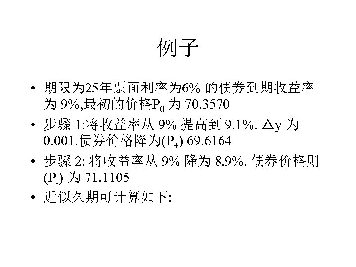
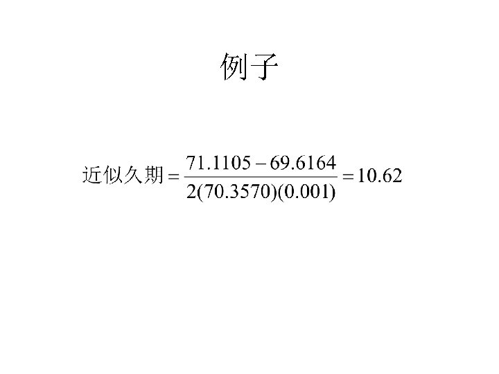
例子 • 期限为 25年票面利率为 6% 的债券到期收益率 为 9%, 最初的价格P 0 为 70. 3570 • 步骤 1: 将收益率从 9% 提高到 9. 1%. △y 为 0. 001. 债券价格降为(P+) 69. 6164 • 步骤 2: 将收益率从 9% 降为 8. 9%. 债券价格则 (P-) 为 71. 1105 • 近似久期可计算如下:
例子
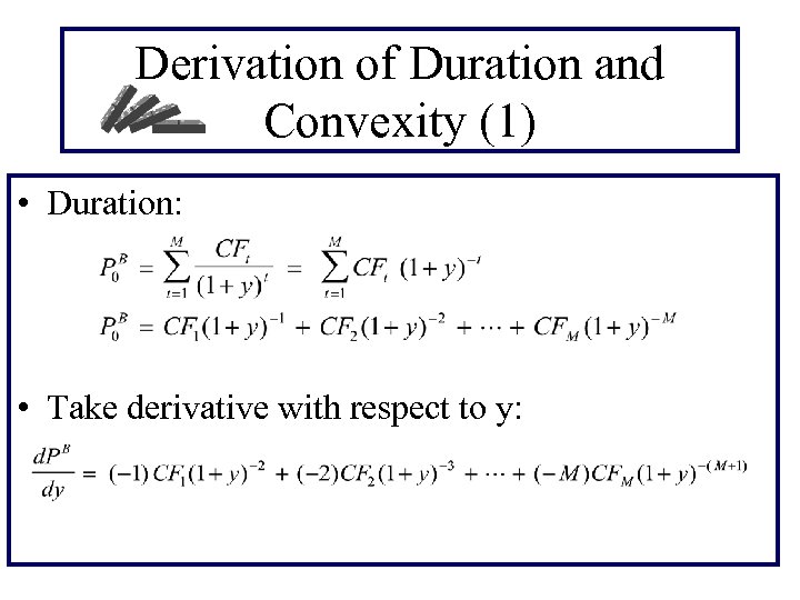
Derivation of Duration and Convexity (1) • Duration: • Take derivative with respect to y:
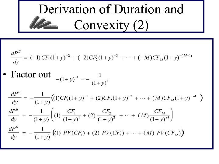
Derivation of Duration and Convexity (2) • Factor out
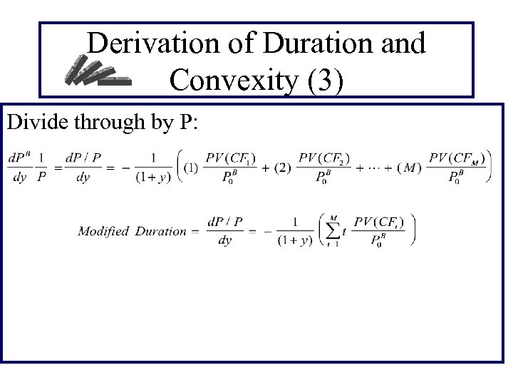
Derivation of Duration and Convexity (3) Divide through by P:
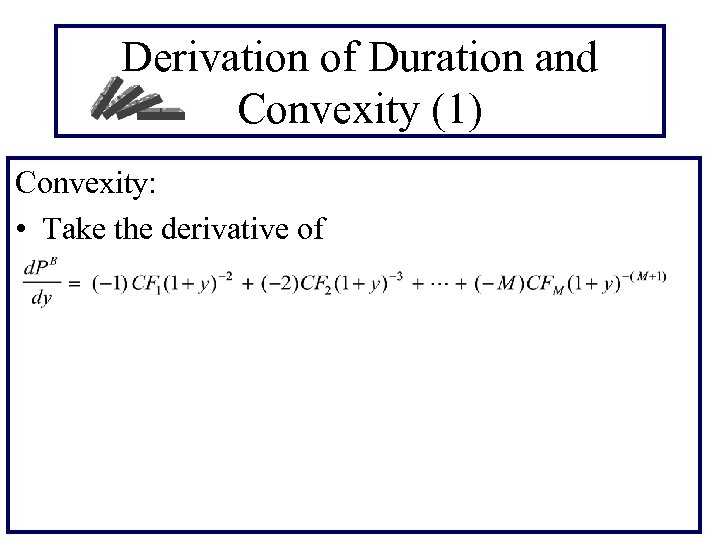
Derivation of Duration and Convexity (1) Convexity: • Take the derivative of
Portfolios • Duration and convexity can be defined similarly for portfolios of bonds and other interest-rate dependent securities • The duration of a portfolio is the weighted average of the durations of the components of the portfolio. Similarly for convexity.
What Duration and Convexity Measure • Duration measures the effect of a small parallel shift in the yield curve • Duration plus convexity measure the effect of a larger parallel shift in the yield curve • However, they do not measure the effect of non-parallel shifts
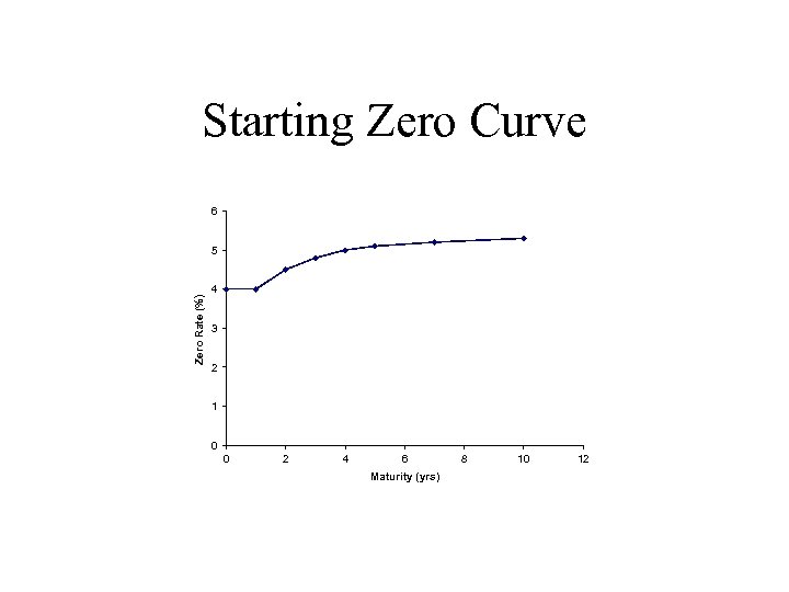
Starting Zero Curve 6 Zero Rate (%) 5 4 3 2 1 0 0 2 4 6 Maturity (yrs) 8 10 12
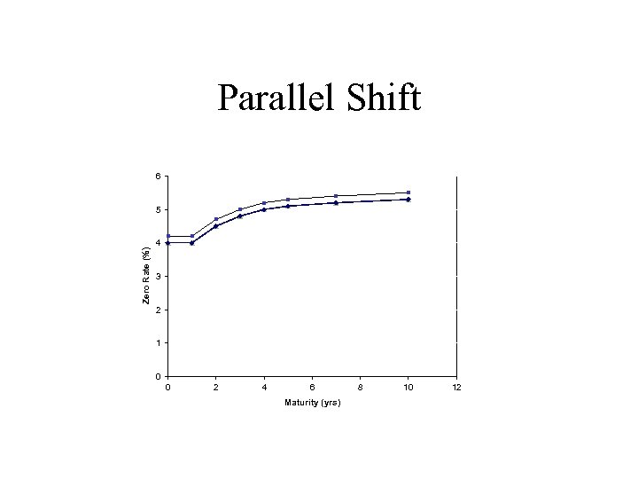
Parallel Shift 6 Zero Rate (%) 5 4 3 2 1 0 0 2 4 6 Maturity (yrs) 8 10 12
Partial Duration • A partial duration calculates the effect on a portfolio of a change to just one point on the zero curve
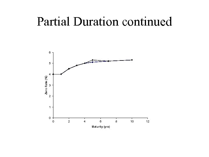
Partial Duration continued 6 Zero Rate (%) 5 4 3 2 1 0 0 2 4 6 Maturity (yrs) 8 10 12
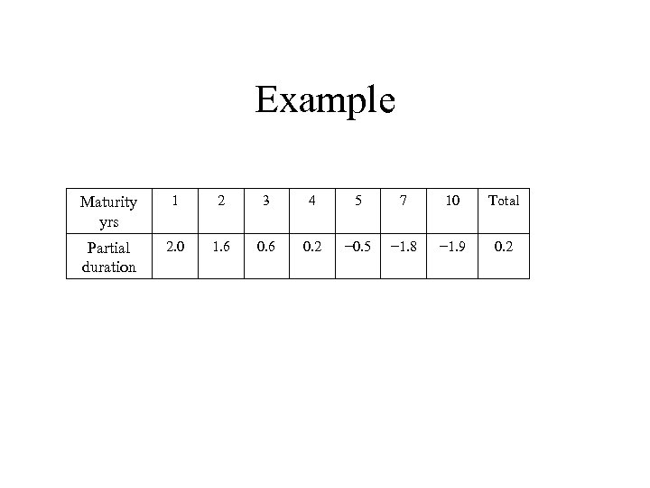
Example Maturity yrs 1 2 3 4 5 7 10 Total Partial duration 2. 0 1. 6 0. 2 − 0. 5 − 1. 8 − 1. 9 0. 2
Partial Durations Can Be Used to Investigate the Impact of Any Yield Curve Change • Any yield curve change can be defined in terms of changes to individual points on the yield curve • For example, to define a rotation we could change the 1 -, 2 -, 3 -, 4 -, 5 -, 7, and 10 -year maturities by − 3 e, − 2 e, − e, 0, e, 3 e, 6 e
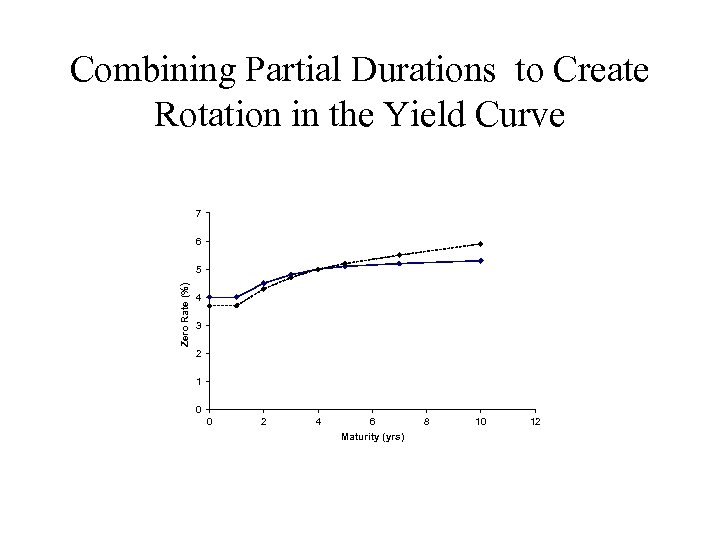
Combining Partial Durations to Create Rotation in the Yield Curve 7 6 Zero Rate (%) 5 4 3 2 1 0 0 2 4 6 Maturity (yrs) 8 10 12
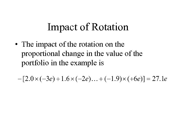
Impact of Rotation • The impact of the rotation on the proportional change in the value of the portfolio in the example is
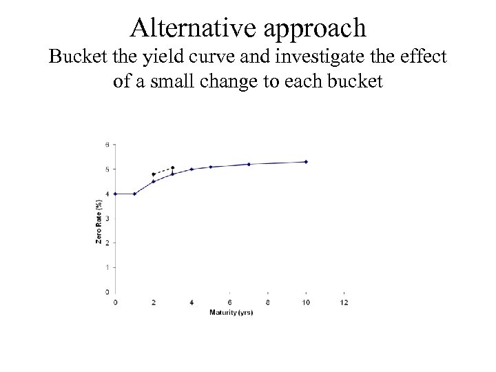
Alternative approach Bucket the yield curve and investigate the effect of a small change to each bucket
Principal Components Analysis • Attempts to identify standard shifts (or factors) for the yield curve so that most of the movements that are observed in practice are combinations of the standard shifts
Historical yield curve movements • Based on USD Treasury rates data between 1989 and 1995, – parallel shift explains 83. 1% of the movements of the yield curve – twist explains 10% of the movements – hump explains 2. 8% of the movements • These three types of movements explain 95. 9% of the movements of the yield curve
DV 01 • DV 01 gives the approximate absolute change in the value of the bond price in response to a 1 basis point change in the yield (typically measured by the ytm of the bond) • The DV 01 of the bond at y=5% is 0. 0779. • for every "small change" in the ytm on the bond. The bond changes by $ 0. 0779.
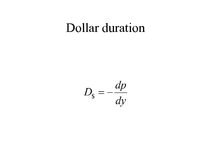
Dollar duration
Definition Va. R is defined as the predicted worst-case loss at a specific confidence level (e. g. 99%) over a certain period of time.
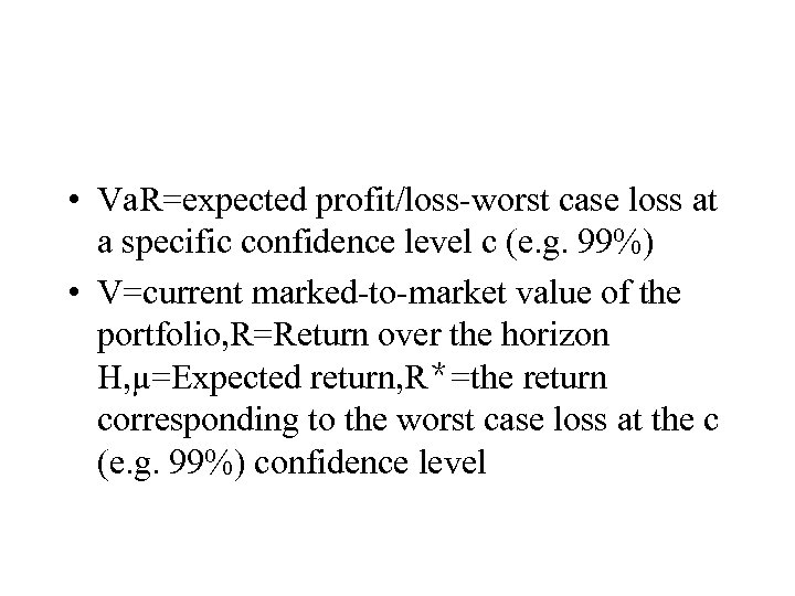
• Va. R=expected profit/loss-worst case loss at a specific confidence level c (e. g. 99%) • V=current marked-to-market value of the portfolio, R=Return over the horizon H, μ=Expected return, R*=the return corresponding to the worst case loss at the c (e. g. 99%) confidence level
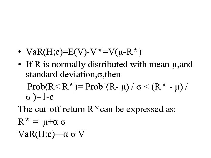
• Va. R(H; c)=E(V)-V*=V(μ-R*) • If R is normally distributed with mean μ, and standard deviation, σ, then Prob(R< R*)= Prob[(R- μ) / σ < (R* - μ) / σ )=1 -c The cut-off return R*can be expressed as: R* = μ+α σ Va. R(H; c)=-α σ V
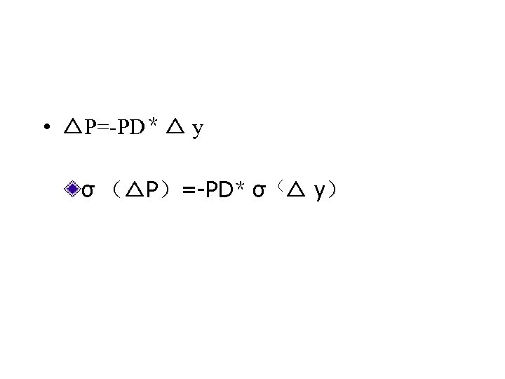
• △P=-PD* △ y σ (△P)=-PD* σ (△ y)
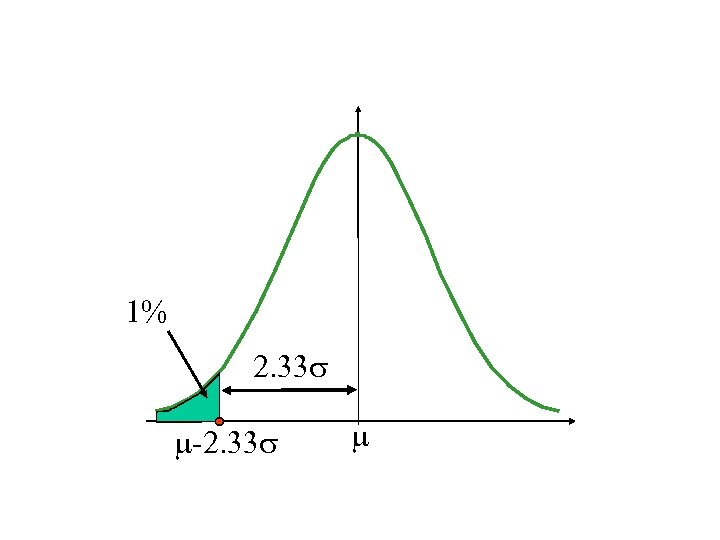
1% 2. 33 -2. 33
7c44680d7710ed6871d70d6085f96975.ppt