FIXED-INCOME SECURITIES Chapter 4 Deriving the Zero-Coupon Yield

FIXED-INCOME SECURITIES Chapter 4 Deriving the Zero-Coupon Yield Curve

Outline • • General Principle Spot Rates Recovering the Term Structure Direct Methods Interpolation Indirect Methods Splines Term Structure of Credit Spreads

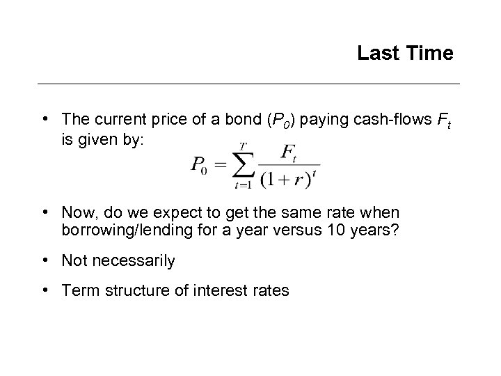Last Time • The current price of a bond (P 0) paying cash-flows Ft is given by: • Now, do we expect to get the same rate when borrowing/lending for a year versus 10 years? • Not necessarily • Term structure of interest rates

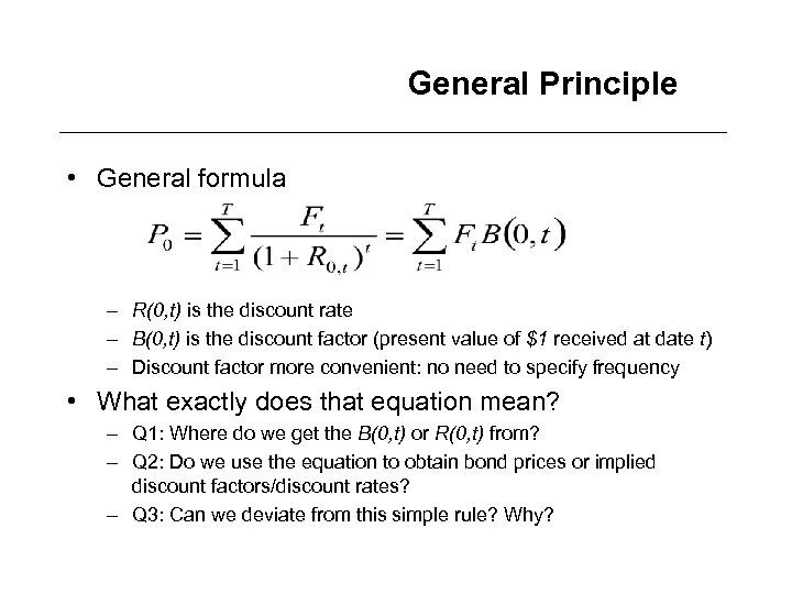General Principle • General formula – R(0, t) is the discount rate – B(0, t) is the discount factor (present value of $1 received at date t) – Discount factor more convenient: no need to specify frequency • What exactly does that equation mean? – Q 1: Where do we get the B(0, t) or R(0, t) from? – Q 2: Do we use the equation to obtain bond prices or implied discount factors/discount rates? – Q 3: Can we deviate from this simple rule? Why?

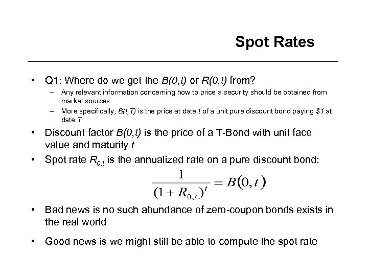Spot Rates • Q 1: Where do we get the B(0, t) or R(0, t) from? – Any relevant information concerning how to price a security should be obtained from market sources – More specifically, B(t, T) is the price at date t of a unit pure discount bond paying $1 at date T • Discount factor B(0, t) is the price of a T-Bond with unit face value and maturity t • Spot rate R 0, t is the annualized rate on a pure discount bond: • Bad news is no such abundance of zero-coupon bonds exists in the real world • Good news is we might still be able to compute the spot rate

Bond Pricing • Answer to the “chicken-and-egg'' second question (Q 2) is – It depends on the situation – Roughly speaking, one would like to use the price of primitive securities as given, and derive implied discount factors or discount rates from them – Then, one may use that information (more specifically the term structure of discount rates) to price any other security – This is known as relative pricing • Answer to the third question (Q 3) is – Any deviation from the pricing rules would imply arbitrage opportunities – Practical illustrations of that concept shall be presented in what follows – Everything we cover in this Chapter can be regarded as some form of perspective on these issues

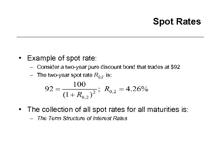Spot Rates • Example of spot rate: – Consider a two-year pure discount bond that trades at $92 – The two-year spot rate R 0, 2 is: • The collection of all spot rates for all maturities is: – The Term Structure of Interest Rates

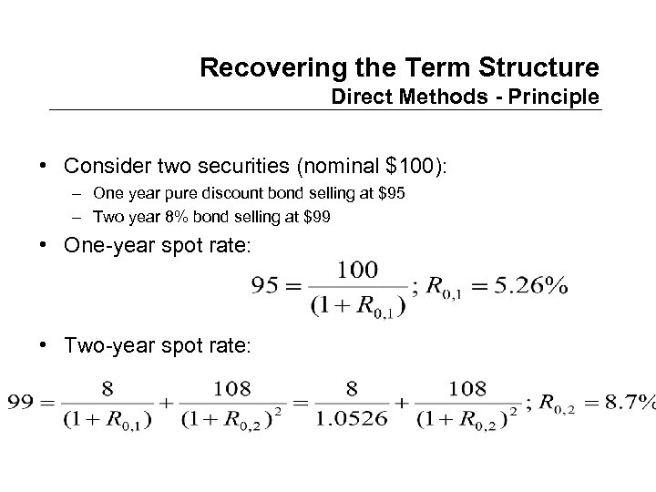Recovering the Term Structure Direct Methods - Principle • Consider two securities (nominal $100): – One year pure discount bond selling at $95 – Two year 8% bond selling at $99 • One-year spot rate: • Two-year spot rate:

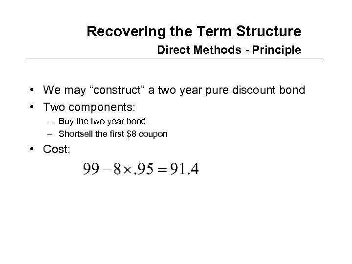Recovering the Term Structure Direct Methods - Principle • We may “construct” a two year pure discount bond • Two components: – Buy the two year bond – Shortsell the first $8 coupon • Cost:

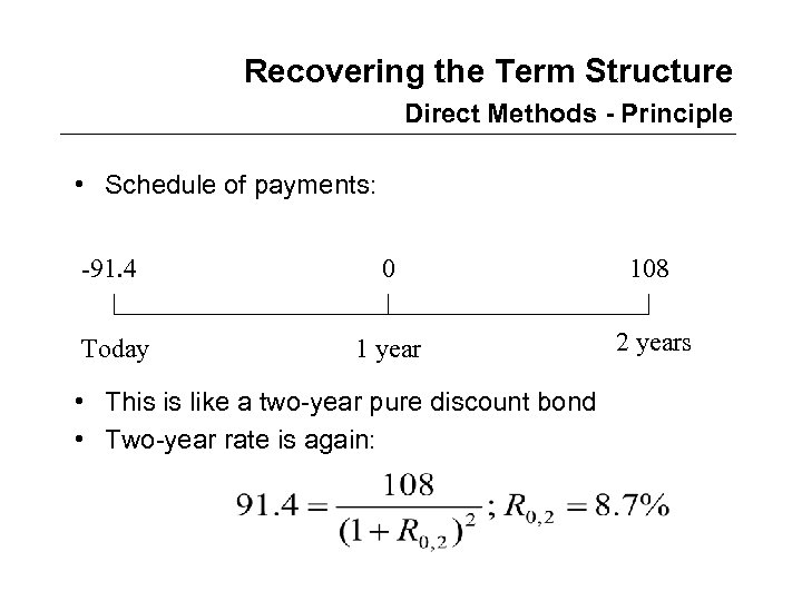Recovering the Term Structure Direct Methods - Principle • Schedule of payments: -91. 4 0 108 Today 1 year 2 years • This is like a two-year pure discount bond • Two-year rate is again:

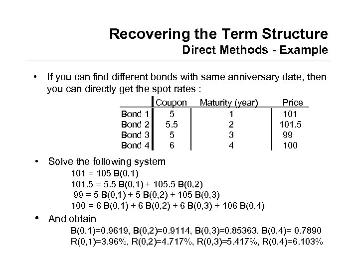Recovering the Term Structure Direct Methods - Example • If you can find different bonds with same anniversary date, then you can directly get the spot rates : Bond 1 Bond 2 Bond 3 Bond 4 Coupon 5 5 6 Maturity (year) 1 2 3 4 Price 101. 5 99 100 • Solve the following system 101 = 105 B(0, 1) 101. 5 = 5. 5 B(0, 1) + 105. 5 B(0, 2) 99 = 5 B(0, 1) + 5 B(0, 2) + 105 B(0, 3) 100 = 6 B(0, 1) + 6 B(0, 2) + 6 B(0, 3) + 106 B(0, 4) • And obtain B(0, 1)=0. 9619, B(0, 2)=0. 9114, B(0, 3)=0. 85363, B(0, 4)= 0. 7890 R(0, 1)=3. 96%, R(0, 2)=4. 717%, R(0, 3)=5. 417%, R(0, 4)=6. 103%

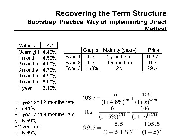Recovering the Term Structure Bootstrap: Practical Way of Implementing Direct Method Maturity Overnight 1 month 2 months 3 months 6 months 9 months 1 year ZC 4. 40% 4. 50% 4. 60% 4. 70% 4. 90% 5. 00% 5. 10% Coupon Maturity (years) Bond 1 5% 1 y and 2 m Bond 2 6% 1 y and 9 m Bond 3 5. 50% 2 y • 1 year and 2 months rate x=5. 41% • 1 year and 9 months rate y= 5. 69% • 2 year rate z= 5. 69% Price 103. 7 102 99. 5

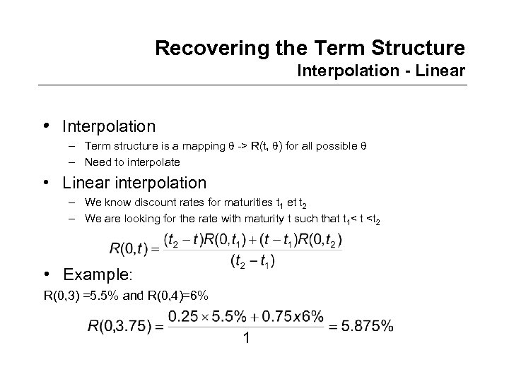Recovering the Term Structure Interpolation - Linear • Interpolation – Term structure is a mapping -> R(t, ) for all possible – Need to interpolate • Linear interpolation – We know discount rates for maturities t 1 et t 2 – We are looking for the rate with maturity t such that t 1< t

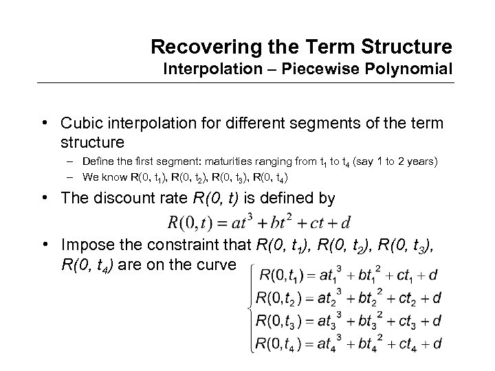Recovering the Term Structure Interpolation – Piecewise Polynomial • Cubic interpolation for different segments of the term structure – Define the first segment: maturities ranging from t 1 to t 4 (say 1 to 2 years) – We know R(0, t 1), R(0, t 2), R(0, t 3), R(0, t 4) • The discount rate R(0, t) is defined by • Impose the constraint that R(0, t 1), R(0, t 2), R(0, t 3), R(0, t 4) are on the curve

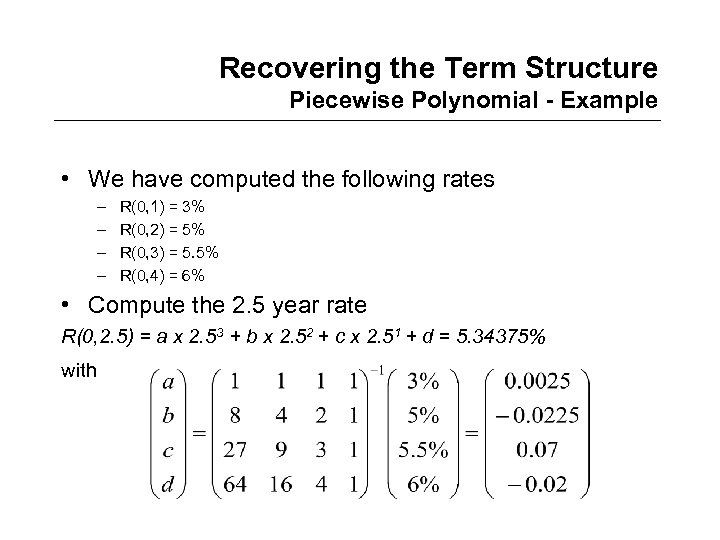Recovering the Term Structure Piecewise Polynomial - Example • We have computed the following rates – – R(0, 1) = 3% R(0, 2) = 5% R(0, 3) = 5. 5% R(0, 4) = 6% • Compute the 2. 5 year rate R(0, 2. 5) = a x 2. 53 + b x 2. 52 + c x 2. 51 + d = 5. 34375% with

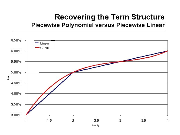Recovering the Term Structure Piecewise Polynomial versus Piecewise Linear 6. 50% Linear Cubic 6. 00% 5. 50% Rate 5. 00% 4. 50% 4. 00% 3. 50% 3. 00% 1 1. 5 2 2. 5 Maturity 3 3. 5 4

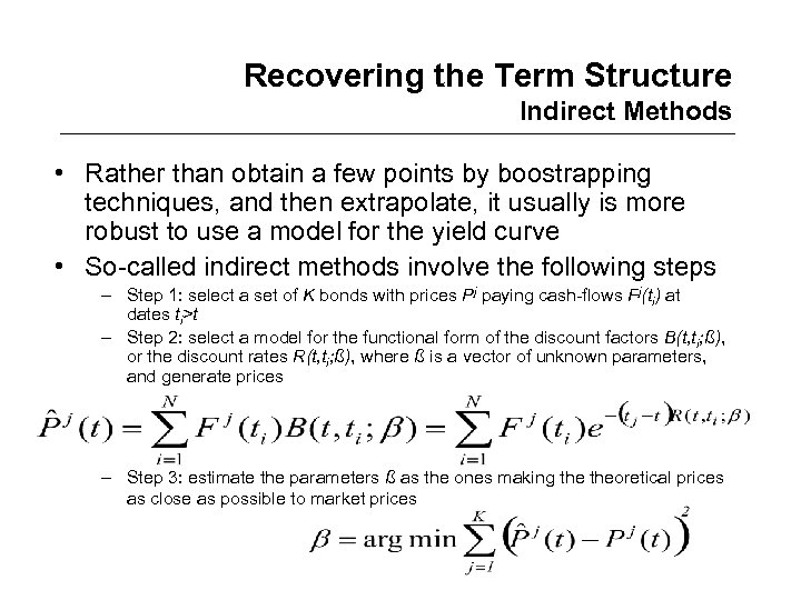Recovering the Term Structure Indirect Methods • Rather than obtain a few points by boostrapping techniques, and then extrapolate, it usually is more robust to use a model for the yield curve • So-called indirect methods involve the following steps – Step 1: select a set of K bonds with prices Pj paying cash-flows Fj(ti) at dates ti>t – Step 2: select a model for the functional form of the discount factors B(t, ti; ß), or the discount rates R(t, ti; ß), where ß is a vector of unknown parameters, and generate prices – Step 3: estimate the parameters ß as the ones making theoretical prices as close as possible to market prices

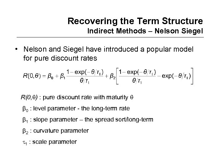Recovering the Term Structure Indirect Methods – Nelson Siegel • Nelson and Siegel have introduced a popular model for pure discount rates R(0, ) : pure discount rate with maturity 0 : level parameter - the long-term rate 1 : slope parameter – the spread sort/long-term 2 : curvature parameter 1 : scale parameter

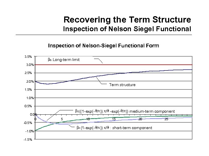Recovering the Term Structure Inspection of Nelson Siegel Functional Inspection of Nelson-Siegel Functional Form 3. 5% 0: Long-term limit 3. 0% 2. 5% 2. 0% Term structure 1. 5% 1. 0% 0. 5% 0. 0% 0 -0. 5% -1. 0% -1. 5% 2 ((1 -exp(- / )). / -exp(- / )) medium-term component 5 10 15 20 1 (1 -exp(- / )). / : short-term component 25

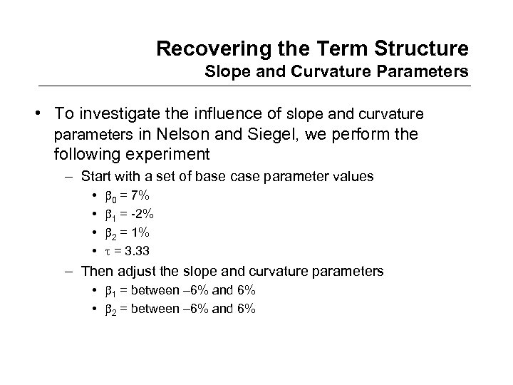Recovering the Term Structure Slope and Curvature Parameters • To investigate the influence of slope and curvature parameters in Nelson and Siegel, we perform the following experiment – Start with a set of base case parameter values • • 0 = 7% 1 = -2% 2 = 1% = 3. 33 – Then adjust the slope and curvature parameters • 1 = between – 6% and 6% • 2 = between – 6% and 6%

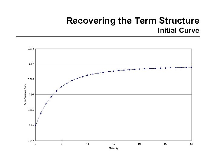Recovering the Term Structure Initial Curve

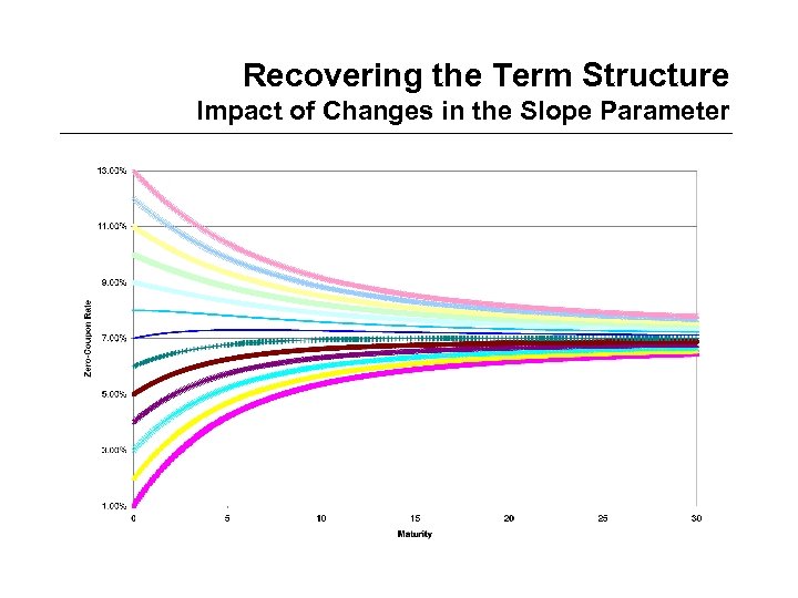Recovering the Term Structure Impact of Changes in the Slope Parameter

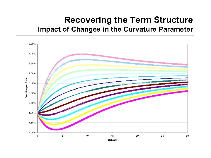Recovering the Term Structure Impact of Changes in the Curvature Parameter

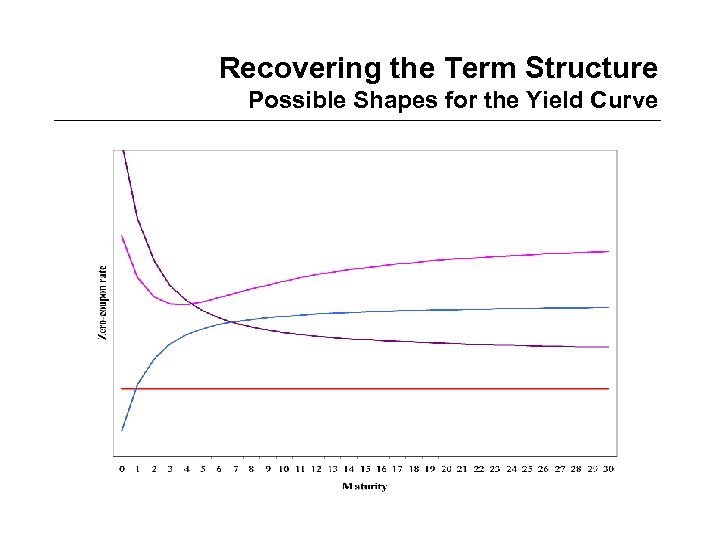Recovering the Term Structure Possible Shapes for the Yield Curve

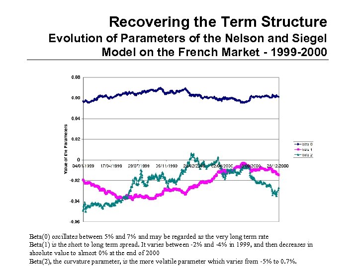Recovering the Term Structure Evolution of Parameters of the Nelson and Siegel Model on the French Market - 1999 -2000 Beta(0) oscillates between 5% and 7% and may be regarded as the very long term rate Beta(1) is the short to long term spread. It varies between -2% and -4% in 1999, and then decreases in absolute value to almost 0% at the end of 2000 Beta(2), the curvature parameter, is the more volatile parameter which varies from -5% to 0. 7%.

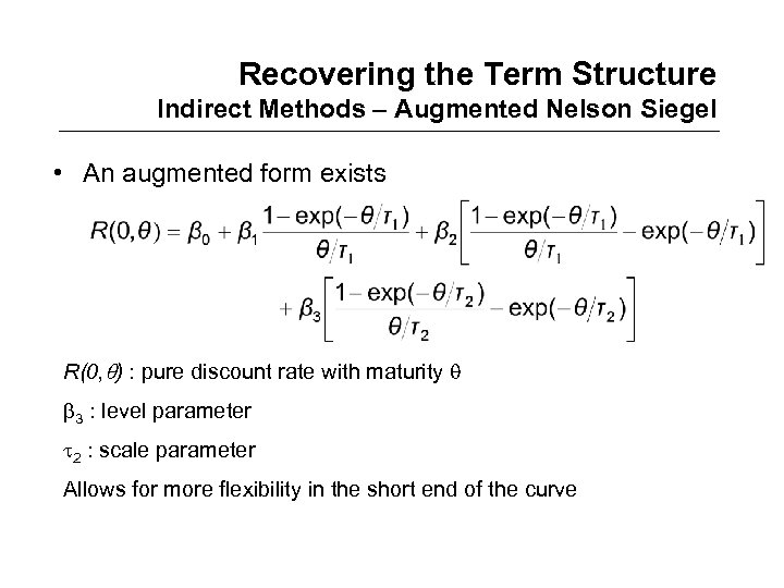Recovering the Term Structure Indirect Methods – Augmented Nelson Siegel • An augmented form exists R(0, ) : pure discount rate with maturity 3 : level parameter 2 : scale parameter Allows for more flexibility in the short end of the curve

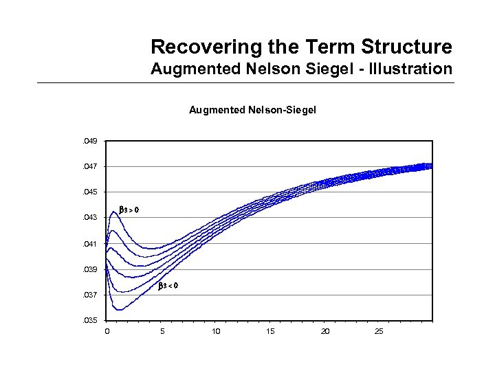Recovering the Term Structure Augmented Nelson Siegel - Illustration Augmented Nelson-Siegel. 049. 047. 045 b 3 > 0 . 043. 041. 039 b 3 < 0 . 037. 035 0 5 10 15 20 25

Recovering the Term Structure Parsimonious Models – Pros and Cons • These models are heavily used in practice • One key advantage is they are parsimonious – Do not involve many parameters – This induces robustness and stability – Very important in the context of hedging • One drawback is their lack of flexibility – Can not account for all possible shapes of the TS we see in practice • Alternative approach: spline models – More flexible – Better for pricing – Less parsimonious • Spline models come in different shapes – Cubic splines – Exponential splines – B-splines

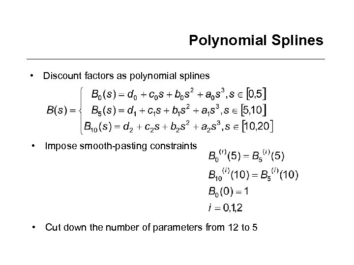Polynomial Splines • Discount factors as polynomial splines • Impose smooth-pasting constraints • Cut down the number of parameters from 12 to 5

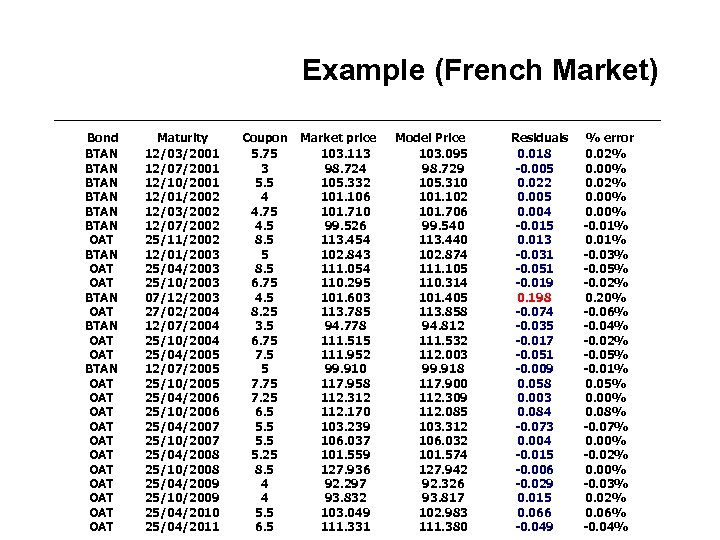Example (French Market) Bond BTAN BTAN OAT OAT BTAN OAT OAT OAT Maturity 12/03/2001 12/07/2001 12/10/2001 12/01/2002 12/03/2002 12/07/2002 25/11/2002 12/01/2003 25/04/2003 25/10/2003 07/12/2003 27/02/2004 12/07/2004 25/10/2004 25/04/2005 12/07/2005 25/10/2005 25/04/2006 25/10/2006 25/04/2007 25/10/2007 25/04/2008 25/10/2008 25/04/2009 25/10/2009 25/04/2010 25/04/2011 Coupon 5. 75 3 5. 5 4 4. 75 4. 5 8. 5 6. 75 4. 5 8. 25 3. 5 6. 75 7. 5 5 7. 75 7. 25 6. 5 5. 25 8. 5 4 4 5. 5 6. 5 Market price 103. 113 98. 724 105. 332 101. 106 101. 710 99. 526 113. 454 102. 843 111. 054 110. 295 101. 603 113. 785 94. 778 111. 515 111. 952 99. 910 117. 958 112. 312 112. 170 103. 239 106. 037 101. 559 127. 936 92. 297 93. 832 103. 049 111. 331 Model Price 103. 095 98. 729 105. 310 101. 102 101. 706 99. 540 113. 440 102. 874 111. 105 110. 314 101. 405 113. 858 94. 812 111. 532 112. 003 99. 918 117. 900 112. 309 112. 085 103. 312 106. 032 101. 574 127. 942 92. 326 93. 817 102. 983 111. 380 Residuals 0. 018 -0. 005 0. 022 0. 005 0. 004 -0. 015 0. 013 -0. 031 -0. 051 -0. 019 0. 198 -0. 074 -0. 035 -0. 017 -0. 051 -0. 009 0. 058 0. 003 0. 084 -0. 073 0. 004 -0. 015 -0. 006 -0. 029 0. 015 0. 066 -0. 049 % error 0. 02% 0. 00% -0. 01% -0. 03% -0. 05% -0. 02% 0. 20% -0. 06% -0. 04% -0. 02% -0. 05% -0. 01% 0. 05% 0. 00% 0. 08% -0. 07% 0. 00% -0. 02% 0. 00% -0. 03% 0. 02% 0. 06% -0. 04%

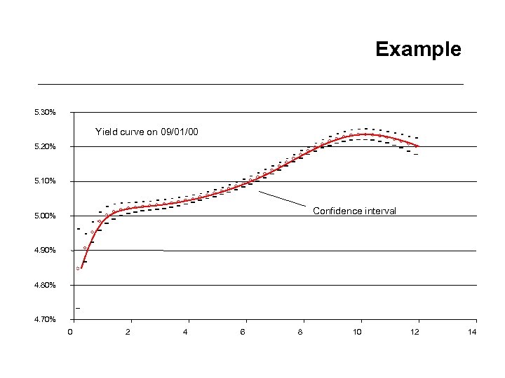Example 5. 30% Yield curve on 09/01/00 5. 20% 5. 10% Confidence interval 5. 00% 4. 90% 4. 80% 4. 70% 0 2 4 6 8 10 12 14