7c81ab22fc50d69d90ac99e7c2bc2b0e.ppt
- Количество слайдов: 23
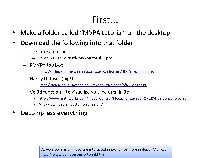 First. . . • Make a folder called “MVPA tutorial” on the desktop • Download the following into that folder: – This presentation – psy 2. ucsd. edu/~crieth/MVPAtutorial_3. ppt – PMVPA toolbox – http: //princeton-mvpa-toolbox. googlecode. com/files/mvpa 1. 1. tar. gz – Haxby Dataset (big!) – http: //www. pni. princeton. edu/mvpa/downloads/afni_set. tar. gz – Vol 3 d function – to visualize volume data in 3 d • http: //www. mathworks. com/matlabcentral/fileexchange/22940 -vol 3 d-v 2/content/vol 3 d. m • (click download all button on the right) • Decompress everything At your own risk. . . if you are interested in python or more in depth MVPA. . . http: //www. pymvpa. org/tutorial. html
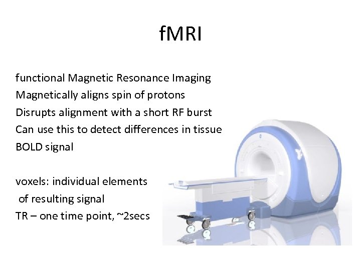 f. MRI functional Magnetic Resonance Imaging Magnetically aligns spin of protons Disrupts alignment with a short RF burst Can use this to detect differences in tissue BOLD signal voxels: individual elements of resulting signal TR – one time point, ~2 secs
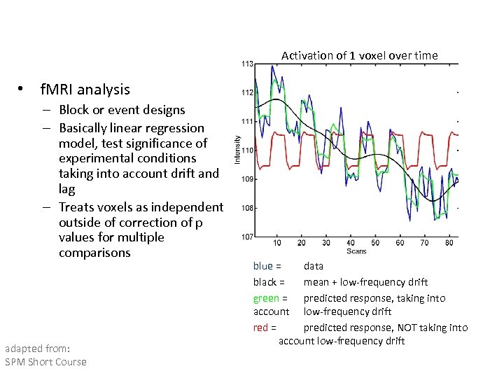 Activation of 1 voxel over time • f. MRI analysis – Block or event designs – Basically linear regression model, test significance of experimental conditions taking into account drift and lag – Treats voxels as independent outside of correction of p values for multiple comparisons adapted from: SPM Short Course blue = data black = mean + low-frequency drift green = predicted response, taking into account low-frequency drift red = predicted response, NOT taking into account low-frequency drift
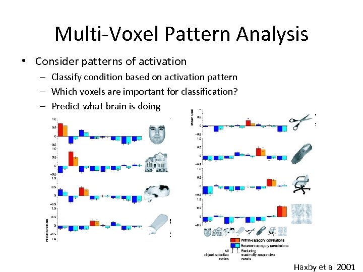 Multi-Voxel Pattern Analysis • Consider patterns of activation – Classify condition based on activation pattern – Which voxels are important for classification? – Predict what brain is doing Haxby et al 2001
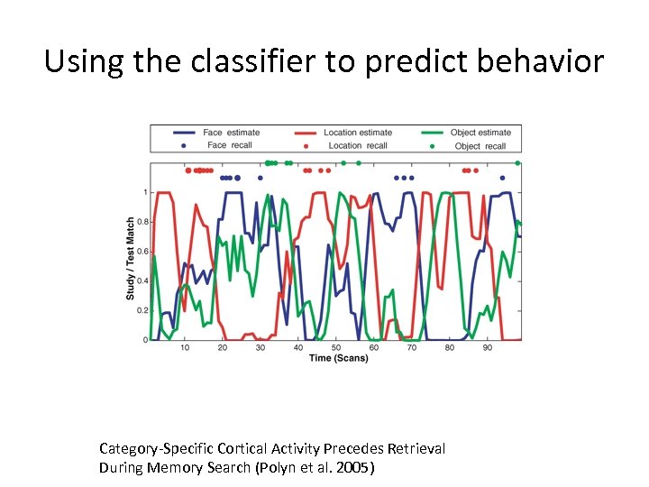 Using the classifier to predict behavior Category-Specific Cortical Activity Precedes Retrieval During Memory Search (Polyn et al. 2005)
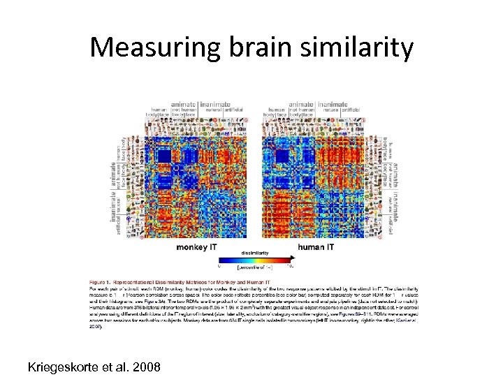 Measuring brain similarity Kriegeskorte et al. 2008
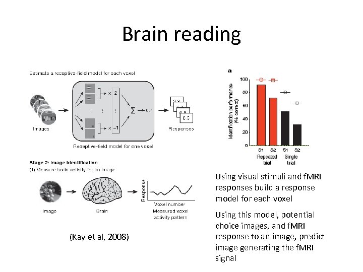 Brain reading Using visual stimuli and f. MRI responses build a response model for each voxel (Kay et al, 2008) Using this model, potential choice images, and f. MRI response to an image, predict image generating the f. MRI signal
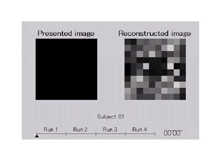
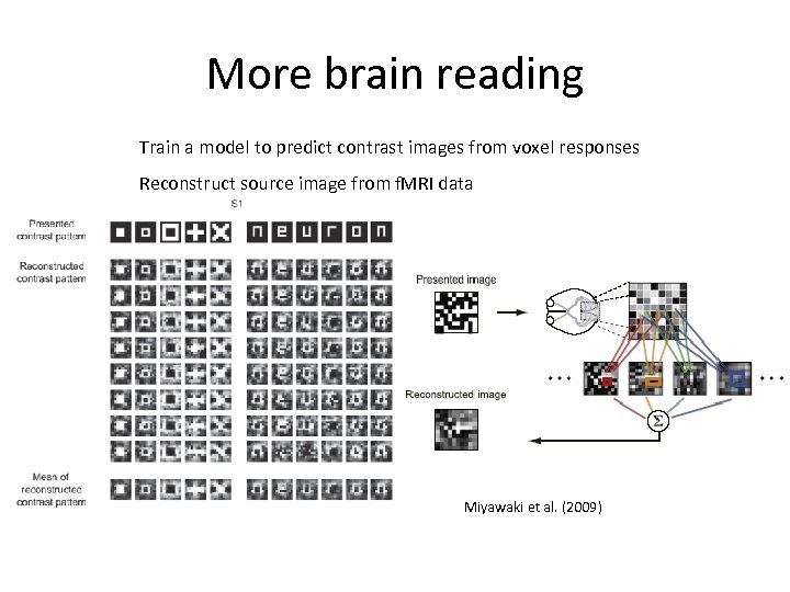 More brain reading Train a model to predict contrast images from voxel responses Reconstruct source image from f. MRI data Miyawaki et al. (2009)
 Nishimoto et al 2011
 Today's objectives • Get hands dirty with some basic MVPA – – – Build confidence in Matlab/programming/exploring code Understand the tutorial code Understand the importance of cross-validation Classify between conditions View f. MRI data in matlab Super bonus round! – Try different classifiers – Examine learned classifier – Measure voxel importance
 Using Princeton Multi Voxel Pattern Analysis Toolbox If interested in MVPA, it is worth reading through their toolbox tutorial in more detail https: //code. google. com/p/princeton-mvpatoolbox/wiki/Tutorial. Intro
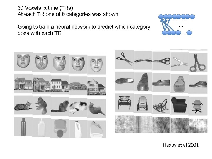 3 d Voxels x time (TRs) At each TR one of 8 categories was shown Going to train a neural network to predict which category goes with each TR . . . Haxby et al 2001
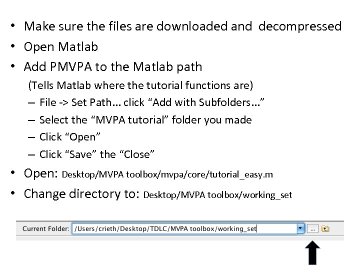 • Make sure the files are downloaded and decompressed • Open Matlab • Add PMVPA to the Matlab path (Tells Matlab where the tutorial functions are) – File -> Set Path. . . click “Add with Subfolders. . . ” – Select the “MVPA tutorial” folder you made – Click “Open” – Click “Save” the “Close” • Open: Desktop/MVPA toolbox/mvpa/core/tutorial_easy. m • Change directory to: Desktop/MVPA toolbox/working_set
 • (To really understand what is going on, it is worth reading through the tutorial code and website explaining it) • For now, on the command line, type: [subj results] = tutorial_easy() This will run the tutorial code, which loads in 10 session of data, masks the patterns to only include IT, preprocesses the data, trains a neural network to classify the different categories using cross validation, and stores the results in a variable called. . . wait for it. . . results. (Matlab will print out a number of warnings, ok to ignore for now) • The average accuracy is given in results. total_perf • Is this accuracy ‘good’? What is chance?
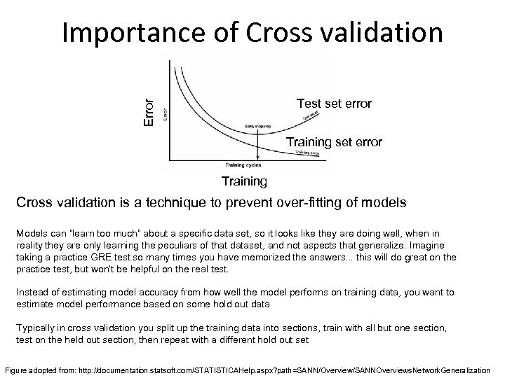 Importance of Cross validation Error Test set error Training Cross validation is a technique to prevent over-fitting of models Models can “learn too much” about a specific data set, so it looks like they are doing well, when in reality they are only learning the peculiars of that dataset, and not aspects that generalize. Imagine taking a practice GRE test so many times you have memorized the answers. . . this will do great on the practice test, but won’t be helpful on the real test. Instead of estimating model accuracy from how well the model performs on training data, you want to estimate model performance based on some hold out data Typically in cross validation you split up the training data into sections, train with all but one section, test on the held out section, then repeat with a different hold out set Figure adopted from: http: //documentation. statsoft. com/STATISTICAHelp. aspx? path=SANN/Overview/SANNOverviews. Network. Generalization
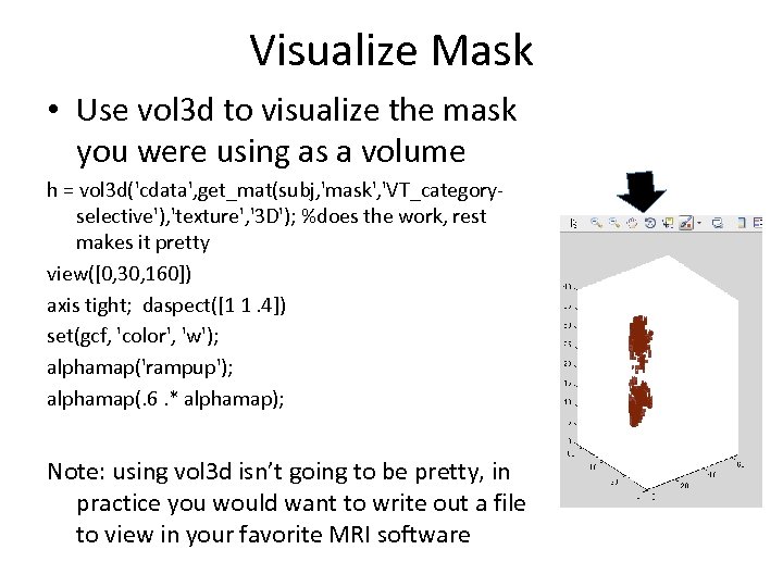 Visualize Mask • Use vol 3 d to visualize the mask you were using as a volume h = vol 3 d('cdata', get_mat(subj, 'mask', 'VT_categoryselective'), 'texture', '3 D'); %does the work, rest makes it pretty view([0, 30, 160]) axis tight; daspect([1 1. 4]) set(gcf, 'color', 'w'); alphamap('rampup'); alphamap(. 6. * alphamap); Note: using vol 3 d isn’t going to be pretty, in practice you would want to write out a file to view in your favorite MRI software
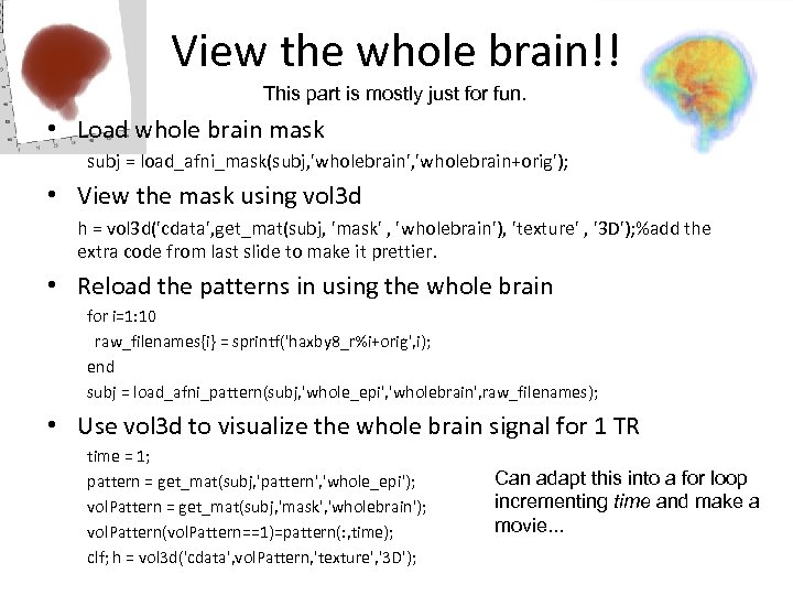 View the whole brain!! This part is mostly just for fun. • Load whole brain mask subj = load_afni_mask(subj, 'wholebrain', 'wholebrain+orig'); • View the mask using vol 3 d h = vol 3 d('cdata', get_mat(subj, 'mask' , 'wholebrain'), 'texture' , '3 D'); %add the extra code from last slide to make it prettier. • Reload the patterns in using the whole brain for i=1: 10 raw_filenames{i} = sprintf('haxby 8_r%i+orig', i); end subj = load_afni_pattern(subj, 'whole_epi', 'wholebrain', raw_filenames); • Use vol 3 d to visualize the whole brain signal for 1 TR time = 1; pattern = get_mat(subj, 'pattern', 'whole_epi'); vol. Pattern = get_mat(subj, 'mask', 'wholebrain'); vol. Pattern(vol. Pattern==1)=pattern(: , time); clf; h = vol 3 d('cdata', vol. Pattern, 'texture', '3 D'); Can adapt this into a for loop incrementing time and make a movie. . .
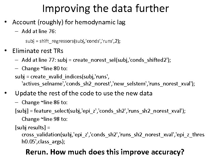 Improving the data further • Account (roughly) for hemodynamic lag – Add at line 76: subj = shift_regressors(subj, 'conds', 'runs', 2); • Eliminate rest TRs – Add at line 77: subj = create_norest_sel(subj, 'conds_shifted 2'); – Change ~line 80 to: subj = create_xvalid_indices(subj, 'runs', 'actives_selname', 'conds_sh 2_norest', 'new_selstem', 'runs_norest_xval'); • Update the rest of the code to use the new data – Change ~line 86 to: [subj] = feature_select(subj, 'epi_z', 'conds_sh 2', 'runs_sh 2_norest_xval'); Change ~line 98 to: [subj results] = cross_validation(subj, 'epi_z', 'conds_sh 2', 'runs_sh 2_norest_xval', 'epi_z_thres h 0. 05', class_args); Rerun. How much does this improve accuracy?
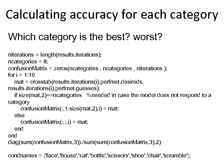 Calculating accuracy for each category Which category is the best? worst? niterations = length(results. iterations); ncategories = 8; confusion. Matrix = zeros(ncategories , niterations ); for i = 1: 10 mat = crosstab(results. iterations(i). perfmet. desireds, results. iterations(i). perfmet. guesses); if size(mat, 2)~=ncategories %needed in case the model does not respond to a category confusion. Matrix(: , 1: size(mat, 2), i) = mat; else confusion. Matrix(: , i) = mat; end diag(sum(confusion. Matrix, 3)). /sum(confusion. Matrix, 3), 2) condnames = {'face', 'house', 'cat', 'bottle', 'scissors', 'shoe', 'chair', 'scramble'};
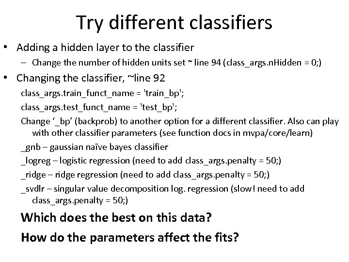 Try different classifiers • Adding a hidden layer to the classifier – Change the number of hidden units set ~ line 94 (class_args. n. Hidden = 0; ) • Changing the classifier, ~line 92 class_args. train_funct_name = 'train_bp'; class_args. test_funct_name = 'test_bp'; Change ‘_bp’ (backprob) to another option for a different classifier. Also can play with other classifier parameters (see function docs in mvpa/core/learn) _gnb – gaussian naïve bayes classifier _logreg – logistic regression (need to add class_args. penalty = 50; ) _ridge – ridge regression (need to add class_args. penalty = 50; ) _svdlr – singular value decomposition log. regression (slow! need to add class_args. penalty = 50; ) Which does the best on this data? How do the parameters affect the fits?
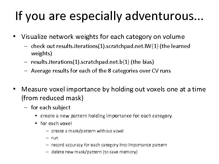 If you are especially adventurous. . . • Visualize network weights for each category on volume – check out results. iterations(1). scratchpad. net. IW{1} (the learned weights) – results. iterations(1). scratchpad. net. b{1} (the bias) – Average results for each of the 8 categories over CV runs • Measure voxel importance by holding out voxels one at a time (from reduced mask) – for each subject • create a new pattern holding importance for each category • for each voxel – – create a mask/pattern without voxel run record accuracy for each category into importance pattern delete new mask/pattern (to save memory)
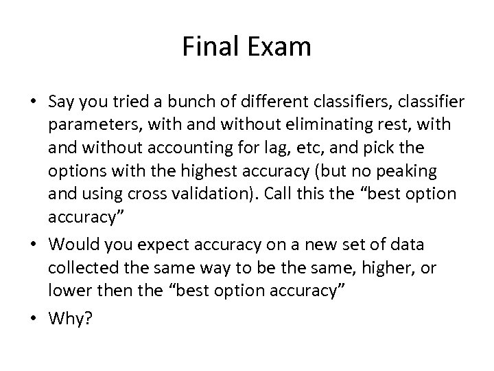 Final Exam • Say you tried a bunch of different classifiers, classifier parameters, with and without eliminating rest, with and without accounting for lag, etc, and pick the options with the highest accuracy (but no peaking and using cross validation). Call this the “best option accuracy” • Would you expect accuracy on a new set of data collected the same way to be the same, higher, or lower then the “best option accuracy” • Why?


