Finite Automata Example 2 Can we build a

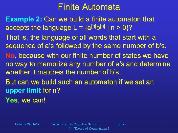
Finite Automata Example 2: Can we build a finite automaton that accepts the language L = {a[n]b[n] | n > 0}? That is, the language of all words that start with a sequence of a’s followed by the same number of b’s. No, because with our finite number of states we have no way to memorize any number of a’s and determine whether it matches the number of b’s. But can we build such an automaton if we set an upper limit for n? Yes, we can! October 29, 2009 Introduction to Cognitive Science 14: Theory of Computation I Lecture 1

Finite Automata Example 3: A finite automaton that accepts L = {a[n]b[n] | 0 < n 2} = {ab, aabb}: q 2 a q 1 a q 3 b b a b q 5 q 6 a, b q 4 a, b October 29, 2009 Introduction to Cognitive Science 14: Theory of Computation I Lecture 2

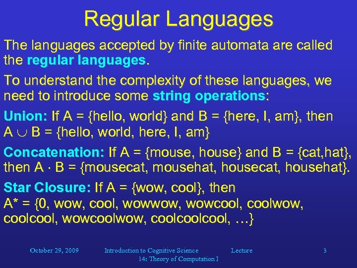
Regular Languages The languages accepted by finite automata are called the regular languages. To understand the complexity of these languages, we need to introduce some string operations: Union: If A = {hello, world} and B = {here, I, am}, then A B = {hello, world, here, I, am} Concatenation: If A = {mouse, house} and B = {cat, hat}, then A B = {mousecat, mousehat, housecat, househat}. Star Closure: If A = {wow, cool}, then A* = {0, wow, cool, wowwow, wowcool, coolwow, cool, wowcoolwow, coolcool, …} October 29, 2009 Introduction to Cognitive Science 14: Theory of Computation I Lecture 3

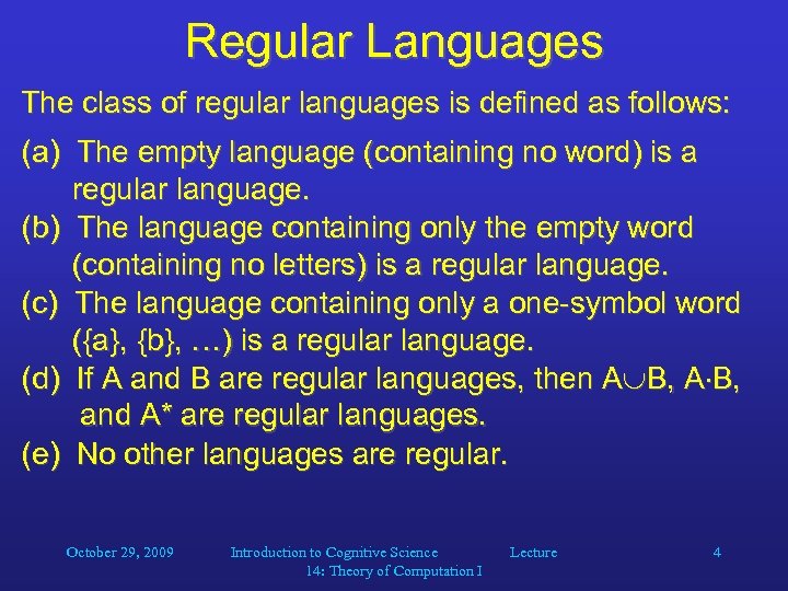
Regular Languages The class of regular languages is defined as follows: (a) The empty language (containing no word) is a regular language. (b) The language containing only the empty word (containing no letters) is a regular language. (c) The language containing only a one-symbol word ({a}, {b}, …) is a regular language. (d) If A and B are regular languages, then A B, and A* are regular languages. (e) No other languages are regular. October 29, 2009 Introduction to Cognitive Science 14: Theory of Computation I Lecture 4

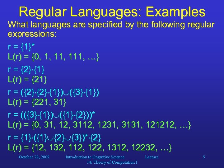
Regular Languages: Examples What languages are specified by the following regular expressions: r = {1}* L(r) = {0, 1, 111, …} r = {2} {1} L(r) = {21} r = ({2} {1}) ({3} {1}) L(r) = {221, 31} r = (({3} {1}) ({1} {2}))* L(r) = {0, 31, 12, 3112, 1231, 3131, 121212, …} r = {1} ({1} {2} {3})* {2} L(r) = {12, 132, 112, 122, 1312, 12232, …} October 29, 2009 Introduction to Cognitive Science 14: Theory of Computation I Lecture 5

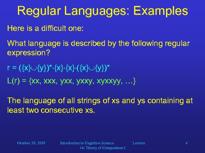
Regular Languages: Examples Here is a difficult one: What language is described by the following regular expression? r = ({x} {y})* {x} ({x} {y})* L(r) = {xx, xxx, yxxy, xyxxyy, …} The language of all strings of xs and ys containing at least two consecutive xs. October 29, 2009 Introduction to Cognitive Science 14: Theory of Computation I Lecture 6

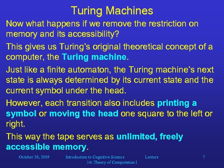
Turing Machines Now what happens if we remove the restriction on memory and its accessibility? This gives us Turing’s original theoretical concept of a computer, the Turing machine. Just like a finite automaton, the Turing machine’s next state is always determined by its current state and the current symbol under the head. However, each transition also includes printing a symbol or moving the head one square to the left or right. This way the tape serves as unlimited, freely accessible memory. October 29, 2009 Introduction to Cognitive Science 14: Theory of Computation I Lecture 7

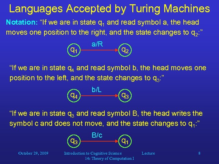
Languages Accepted by Turing Machines Notation: “If we are in state q 1 and read symbol a, the head moves one position to the right, and the state changes to q 2: ” q 1 a/R q 2 “If we are in state q 4 and read symbol b, the head moves one position to the left, and the state changes to q 3: ” q 4 b/L q 3 “If we are in state q 3 and read symbol B, the head writes the symbol c and does not move, and the state changes to q 1: ” q 3 October 29, 2009 B/c q 1 Introduction to Cognitive Science 14: Theory of Computation I Lecture 8

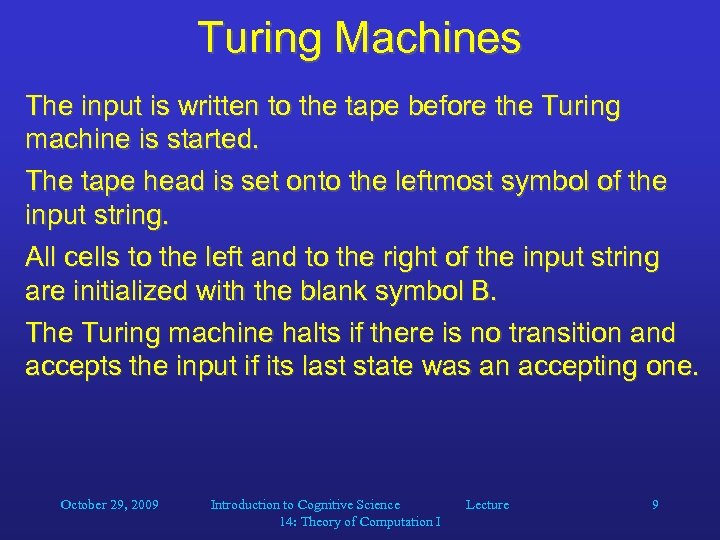
Turing Machines The input is written to the tape before the Turing machine is started. The tape head is set onto the leftmost symbol of the input string. All cells to the left and to the right of the input string are initialized with the blank symbol B. The Turing machine halts if there is no transition and accepts the input if its last state was an accepting one. October 29, 2009 Introduction to Cognitive Science 14: Theory of Computation I Lecture 9

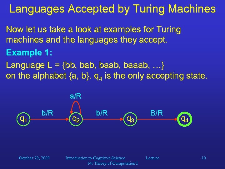
Languages Accepted by Turing Machines Now let us take a look at examples for Turing machines and the languages they accept. Example 1: Language L = {bb, baab, baaab, …} on the alphabet {a, b}. q 4 is the only accepting state. a/R q 1 b/R October 29, 2009 q 2 b/R q 3 Introduction to Cognitive Science 14: Theory of Computation I B/R Lecture q 4 10

Languages Accepted by Turing Machines Example 2: Language L = {a[n]b[n] | n > 0} on the alphabet {a, b}. a/R q 1 a/B q 2 B/R q 3 b/R B/L a/L q 8 b/L October 29, 2009 q 6 B/B B/L q 5 b/B q 4 q 7 Introduction to Cognitive Science 14: Theory of Computation I Lecture 11

TMs as Computers Church’s thesis: Any function that can be algorithmically computed can also be computed by a Turing machine. Why is it only a thesis? There is no general mathematical definition of algorithm – it is always specific to a particular scheme, i. e. , a programming language. Therefore, Church’s thesis cannot be proved. However, no counterexample has been found, and no scientist seriously doubts that Church’s thesis is correct. October 29, 2009 Introduction to Cognitive Science 14: Theory of Computation I Lecture 12