Financial integration and short-run macroeconomic equilibrium Chap

Financial integration and short-run macroeconomic equilibrium § Chap. 16 -17 in the Krugman and Obstfeld textbook § Chap. 22, 23, 24, 25 in the Mishkin textbook § Large capital flows today -> open economies § Consequences of these capital flows on short-run macroeconomic equilibrium Copyright © 2003 Pearson Education, Inc.

Chapter Organization § Determinants of Aggregate Demand in an Open § § § Economy The Equation of Aggregate Demand How Output Is Determined in the Short Run Output Market Equilibrium in the Sort Run: The DD Schedule Asset Market Equilibrium in the Short Run: The AA Schedule Short-Run Equilibrium for an Open Economy: Putting the DD and AA Schedules Together Copyright © 2003 Pearson Education, Inc.

Chapter Organization § Temporary Changes in Monetary and Fiscal Policy § Inflation Bias and Other Problems of Policy § § Formulation Permanent Shifts in Monetary and Fiscal Policy Macroeconomic Policies and the Current Account Gradual Trade Flow Adjustment and Current Account Dynamics Summary Copyright © 2003 Pearson Education, Inc.

Introduction § Macroeconomic changes that affect exchange rates, interest rates, and price levels may also affect output. • This chapter introduces a new theory of how the output market adjusts to demand changes when product prices are themselves slow to adjust. § A short-run model of the output market in an open economy will be utilized to analyze: • The effects of macroeconomic policy tools on output • and the current account The use of macroeconomic policy tools to maintain full employment Copyright © 2003 Pearson Education, Inc.

Determinants of Aggregate Demand in an Open Economy § Aggregate demand • The amount of a country’s goods and services demanded by households and firms throughout the world. § The aggregate demand for an open economy’s output consists of four components: • • Consumption demand (C) Investment demand (I) Government demand (G) Current account (CA) Copyright © 2003 Pearson Education, Inc.

Determinants of Aggregate Demand in an Open Economy § Determinants of Consumption Demand • Consumption demand increases as disposable income (i. e. , national income less taxes) increases at the aggregate level. – The increase in consumption demand is less than the increase in the disposable income because part of the income increase is saved. Copyright © 2003 Pearson Education, Inc.

Determinants of Aggregate Demand in an Open Economy § Determinants of the Current Account • The CA balance is viewed as the demand for a • country’s exports (EX) less that country's own demand for imports (IM). The CA balance is determined by two main factors: – The domestic currency’s real exchange rate against foreign currency (q = EP*/P) – Domestic disposable income (Yd) Copyright © 2003 Pearson Education, Inc.

Determinants of Aggregate Demand in an Open Economy § How Real Exchange Rate Changes Affect the Current Account • An increase in q raises EX and improves the domestic country’s CA. – Each unit of domestic output now purchases fewer units of foreign output, therefore, foreign will demand more exports. • An increase q can raise or lower IM and has an ambiguous effect on CA. – IM denotes the value of imports measured in terms of domestic output. Copyright © 2003 Pearson Education, Inc.

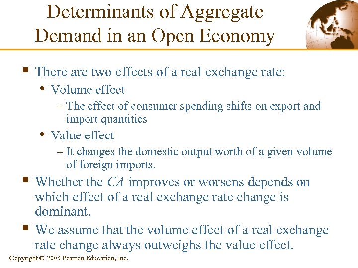
Determinants of Aggregate Demand in an Open Economy § There are two effects of a real exchange rate: • Volume effect – The effect of consumer spending shifts on export and import quantities • Value effect – It changes the domestic output worth of a given volume of foreign imports. § Whether the CA improves or worsens depends on § which effect of a real exchange rate change is dominant. We assume that the volume effect of a real exchange rate change always outweighs the value effect. Copyright © 2003 Pearson Education, Inc.

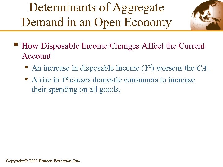
Determinants of Aggregate Demand in an Open Economy § How Disposable Income Changes Affect the Current Account • An increase in disposable income (Yd) worsens the CA. • A rise in Yd causes domestic consumers to increase their spending on all goods. Copyright © 2003 Pearson Education, Inc.

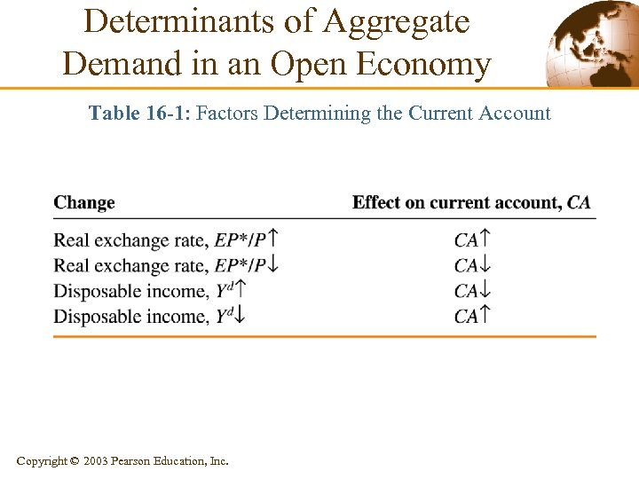
Determinants of Aggregate Demand in an Open Economy Table 16 -1: Factors Determining the

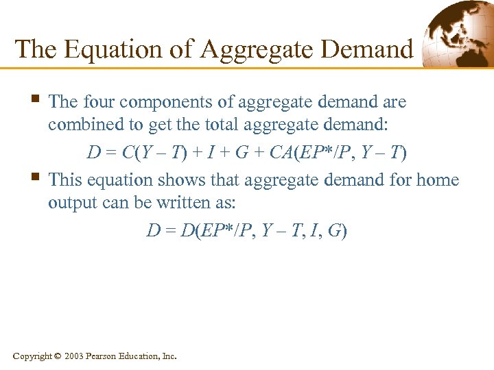
The Equation of Aggregate Demand § The four components of aggregate demand are § combined to get the total aggregate demand: D = C(Y – T) + I + G + CA(EP*/P, Y – T) This equation shows that aggregate demand for home output can be written as: D = D(EP*/P, Y – T, I, G) Copyright © 2003 Pearson Education, Inc.

The Equation of Aggregate Demand § The Real Exchange Rate and Aggregate Demand • An increase in q raises CA and D. – It makes domestic goods and services cheaper relative to foreign goods and services. – It shifts both domestic and foreign spending from foreign goods to domestic goods. – A real depreciation of the home currency raises aggregate demand for home output. – A real appreciation lowers aggregate demand for home output. Copyright © 2003 Pearson Education, Inc.

The Equation of Aggregate Demand § Real Income and Aggregate Demand • A rise in domestic real income raises aggregate • demand for home output. A fall in domestic real income lowers aggregate demand for home output. Copyright © 2003 Pearson Education, Inc.

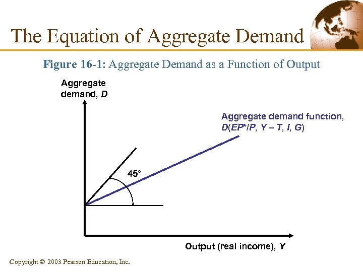
The Equation of Aggregate Demand Figure 16 -1: Aggregate Demand as a Function of Output Aggregate demand, D Aggregate demand function, D(EP*/P, Y – T, I, G) 45° Output (real income), Y Copyright © 2003 Pearson Education, Inc.

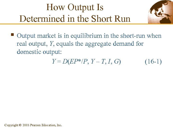
How Output Is Determined in the Short Run § Output market is in equilibrium in the short-run when real output, Y, equals the aggregate demand for domestic output: Y = D(EP*/P, Y – T, I, G) (16 -1) Copyright © 2003 Pearson Education, Inc.

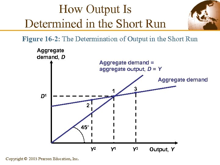
How Output Is Determined in the Short Run Figure 16 -2: The Determination of Output in the Short Run Aggregate demand, D Aggregate demand = aggregate output, D = Y Aggregate demand 1 D 1 3 Y 1 Y 3 2 45° Y 2 Copyright © 2003 Pearson Education, Inc. Output, Y

Output Market Equilibrium in the Short Run: The DD Schedule § Output, the Exchange Rate, and Output Market Equilibrium • With fixed price levels at home and abroad, a rise in the nominal exchange rate makes foreign goods and services more expensive relative to domestic goods and services. – Any rise in q will cause an upward shift in the aggregate demand function and an expansion of output. – Any fall in q will cause output to contract. Copyright © 2003 Pearson Education, Inc.

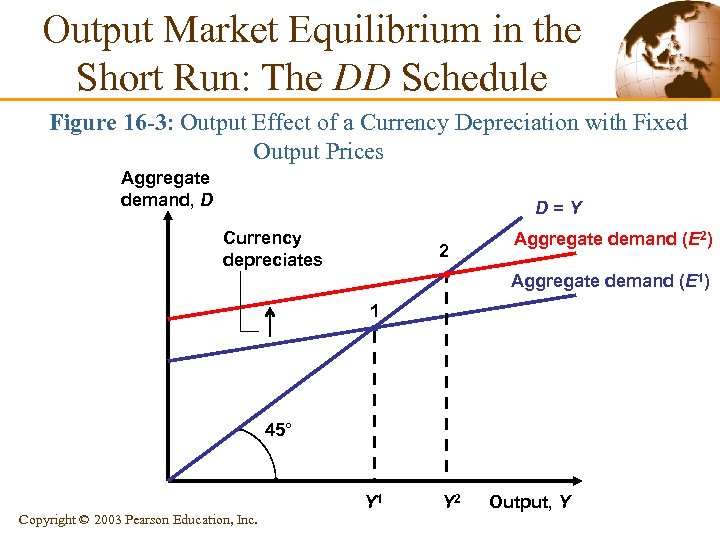
Output Market Equilibrium in the Short Run: The DD Schedule Figure 16 -3: Output Effect of a Currency Depreciation with Fixed Output Prices Aggregate demand, D D=Y Currency depreciates 2 Aggregate demand (E 2) Aggregate demand (E 1) 1 45° Copyright © 2003 Pearson Education, Inc. Y 1 Y 2 Output, Y

Output Market Equilibrium in the Short Run: The DD Schedule § Deriving the DD Schedule • DD schedule – It shows all combinations of output and the exchange rate for which the output market is in short-run equilibrium (aggregate demand = aggregate output). – It slopes upward because a rise in the exchange rate causes output to rise. Copyright © 2003 Pearson Education, Inc.

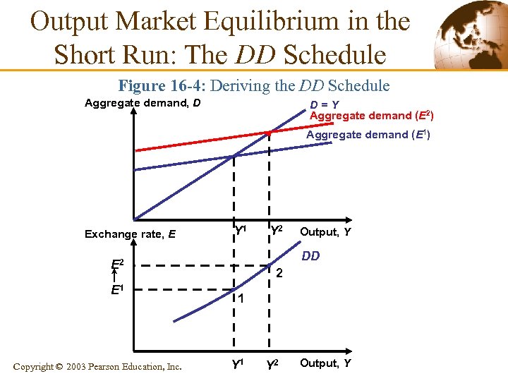
Output Market Equilibrium in the Short Run: The DD Schedule Figure 16 -4: Deriving the DD Schedule Aggregate demand, D D=Y Aggregate demand (E 2) Aggregate demand (E 1) Exchange rate, E Y 1 Copyright © 2003 Pearson Education, Inc. Output, Y DD E 2 E 1 Y 2 2 1 Y 2 Output, Y

Output Market Equilibrium in the Short Run: The DD Schedule § Factors that Shift the DD Schedule • • Government purchases Taxes Investment Domestic price levels Foreign price levels Domestic consumption Demand shift between foreign and domestic goods § A disturbance that raises (lowers) aggregate demand for domestic output shifts the DD schedule to the right (left). Copyright © 2003 Pearson Education, Inc.

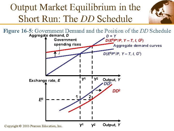
Output Market Equilibrium in the Short Run: The DD Schedule Figure 16 -5: Government Demand the Position of the DD Schedule Aggregate demand, D Government spending rises D=Y D(E 0 P*/P, Y – T, I, G 2) Aggregate demand curves D(E 0 P*/P, Y – T, I, G 1) Y 1 Exchange rate, E Y 2 Output, Y DD 1 DD 2 E 0 Copyright © 2003 Pearson Education, Inc. 1 2 Y 1 Y 2 Output, Y

Asset Market Equilibrium in the Short Run: The AA Schedule § AA Schedule • It shows all combinations of exchange rate and output that are consistent with equilibrium in the domestic money market and the foreign exchange market. Copyright © 2003 Pearson Education, Inc.

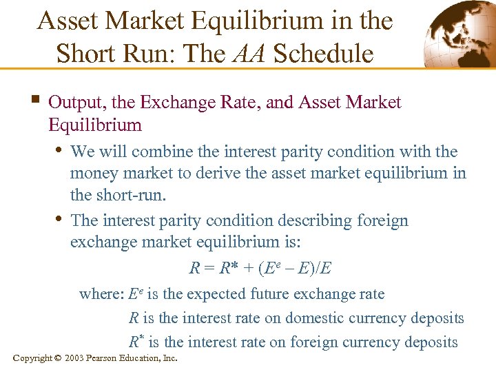
Asset Market Equilibrium in the Short Run: The AA Schedule § Output, the Exchange Rate, and Asset Market Equilibrium • We will combine the interest parity condition with the • money market to derive the asset market equilibrium in the short-run. The interest parity condition describing foreign exchange market equilibrium is: R = R* + (Ee – E)/E where: Ee is the expected future exchange rate R is the interest rate on domestic currency deposits R* is the interest rate on foreign currency deposits Copyright © 2003 Pearson Education, Inc.

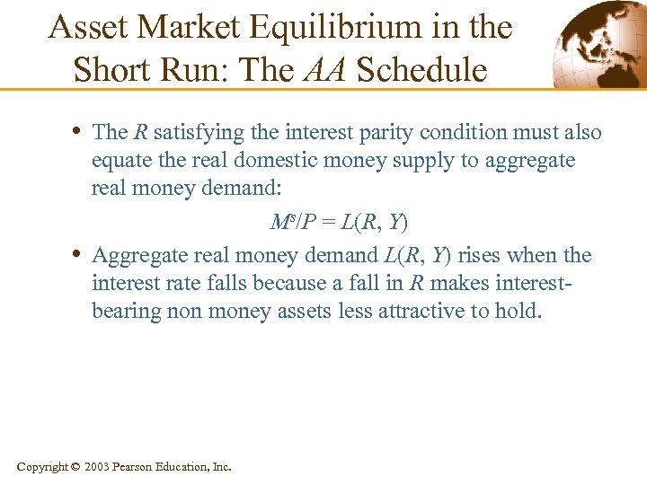
Asset Market Equilibrium in the Short Run: The AA Schedule • The R satisfying the interest parity condition must also • equate the real domestic money supply to aggregate real money demand: Ms/P = L(R, Y) Aggregate real money demand L(R, Y) rises when the interest rate falls because a fall in R makes interestbearing non money assets less attractive to hold. Copyright © 2003 Pearson Education, Inc.

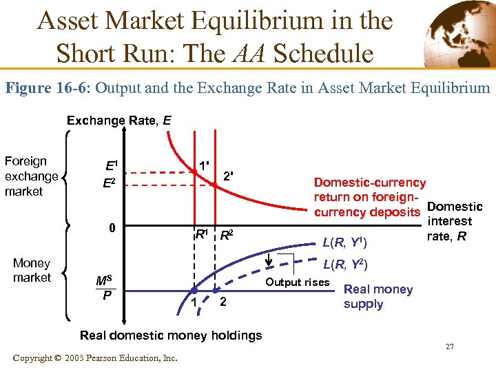
Asset Market Equilibrium in the Short Run: The AA Schedule Figure 16 -6: Output and the Exchange Rate in Asset Market Equilibrium Exchange Rate, E Foreign exchange market 0 Money market 1' E 1 E 2 2' R 1 R 2 Domestic-currency return on foreigncurrency deposits Domestic interest rate, R L(R, Y 1) L(R, Y 2) MS P Output rises 1 2 Real domestic money holdings Copyright © 2003 Pearson Education, Inc. Real money supply 27

Asset Market Equilibrium in the Short Run: The AA Schedule § For asset markets to remain in equilibrium: • A rise in domestic output must be accompanied by an • appreciation of the domestic currency. A fall in domestic output must be accompanied by a depreciation of the domestic currency. Copyright © 2003 Pearson Education, Inc.

Asset Market Equilibrium in the Short Run: The AA Schedule § Deriving the AA Schedule • It relates exchange rates and output levels that keep the • money and foreign exchange markets in equilibrium. It slopes downward because a rise in output causes a rise in the home interest rate and a domestic currency appreciation. Copyright © 2003 Pearson Education, Inc.

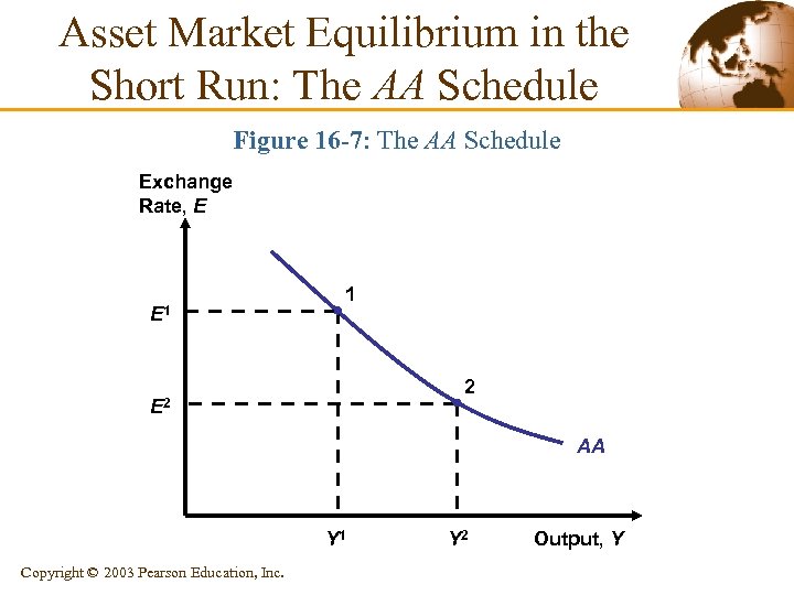
Asset Market Equilibrium in the Short Run: The AA Schedule Figure 16 -7: The

Asset Market Equilibrium in the Short Run: The AA Schedule § Factors that Shift the AA Schedule • • • Domestic money supply Domestic price level Expected future exchange rate Foreign interest rate Shifts in the aggregate real money demand schedule Copyright © 2003 Pearson Education, Inc.

Short-Run Equilibrium for an Open Economy: Putting the DD and AA Schedules Together § A short-run equilibrium for the economy as a whole must bring equilibrium simultaneously in the output and asset markets. • That is, it must lie on both DD and AA schedules. Copyright © 2003 Pearson Education, Inc.

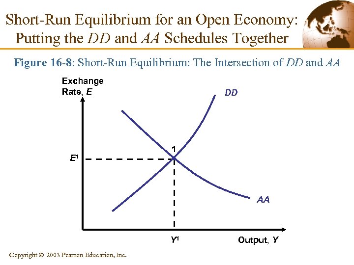
Short-Run Equilibrium for an Open Economy: Putting the DD and AA Schedules Together Figure 16 -8: Short-Run Equilibrium: The Intersection of DD and AA Exchange Rate, E E 1 DD 1 AA Y 1 Copyright © 2003 Pearson Education, Inc. Output, Y

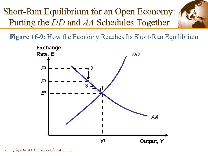
Short-Run Equilibrium for an Open Economy: Putting the DD and AA Schedules Together Figure 16 -9: How the Economy Reaches Its Short-Run Equilibrium Exchange Rate, E DD E 2 E 3 E 1 2 3 1 AA Y 1 Copyright © 2003 Pearson Education, Inc. Output, Y

Temporary Changes in Monetary and Fiscal Policy § Two types of government policy: • Monetary policy – It works through changes in the money supply. • Fiscal policy – It works through changes in government spending or taxes. • Temporary policy shifts are those that the public • expects to be reversed in the near future and do not affect the long-run expected exchange rate. Assume that policy shifts do not influence the foreign interest rate and the foreign price level. Copyright © 2003 Pearson Education, Inc.

Temporary Changes in Monetary and Fiscal Policy § Monetary Policy • An increase in money supply (i. e. , expansionary monetary policy) raises the economy’s output. – The increase in money supply creates an excess supply of money, which lowers the home interest rate. – As a result, the domestic currency must depreciate (i. e. , home products become cheaper relative to foreign products) and aggregate demand increases. Copyright © 2003 Pearson Education, Inc.

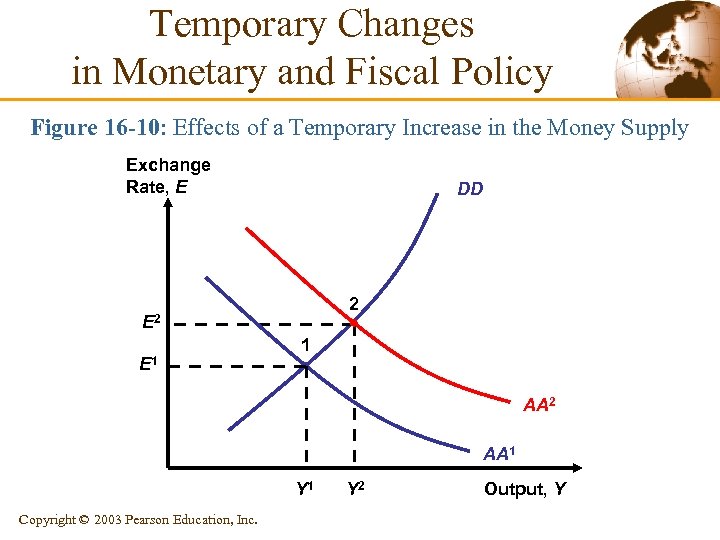
Temporary Changes in Monetary and Fiscal Policy Figure 16 -10: Effects of a Temporary Increase in the Money Supply Exchange Rate, E DD 2 E 1 1 AA 2 AA 1 Y 1 Copyright © 2003 Pearson Education, Inc. Y 2 Output, Y

Temporary Changes in Monetary and Fiscal Policy § Fiscal Policy • An increase in government spending, a cut in taxes, or some combination of the two (i. e, expansionary fiscal policy) raises output. – The increase in output raises the transactions demand for real money holdings, which in turn increases the home interest rate. – As a result, the domestic currency must appreciate. Copyright © 2003 Pearson Education, Inc.

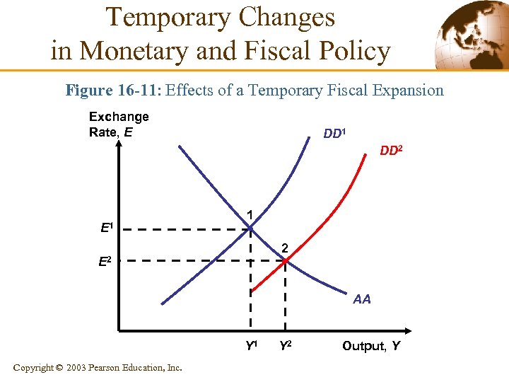
Temporary Changes in Monetary and Fiscal Policy Figure 16 -11: Effects of a Temporary Fiscal Expansion Exchange Rate, E DD 1 DD 2 E 1 1 2 E 2 AA Y 1 Copyright © 2003 Pearson Education, Inc. Y 2 Output, Y

Temporary Changes in Monetary and Fiscal Policy § Policies to Maintain Full Employment • Temporary disturbances that lead to recession can be offset through expansionary monetary or fiscal policies. – Temporary disturbances that lead to overemployment can be offset through contractionary monetary or fiscal policies. Copyright © 2003 Pearson Education, Inc.

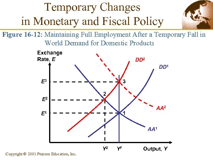
Temporary Changes in Monetary and Fiscal Policy Figure 16 -12: Maintaining Full Employment After a Temporary Fall in World Demand for Domestic Products Exchange Rate, E DD 2 DD 1 E 3 E 2 3 2 1 E 1 AA 2 AA 1 Copyright © 2003 Pearson Education, Inc. Y 2 Yf Output, Y

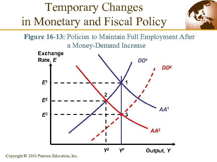
Temporary Changes in Monetary and Fiscal Policy Figure 16 -13: Policies to Maintain Full Employment After a Money-Demand Increase Exchange Rate, E DD 1 DD 2 E 1 E 2 1 2 3 E 3 AA 1 AA 2 Y 2 Copyright © 2003 Pearson Education, Inc. Yf Output, Y

Permanent Shifts in Monetary and Fiscal Policy § A permanent policy shift affects not only the current value of the government’s policy instrument but also the long-run exchange rate. • This affects expectations about future exchange rates. § A Permanent Increase in the Money Supply • A permanent increase in the money supply causes the expected future exchange rate to rise proportionally. – As a result, the upward shift in the AA schedule is greater than that caused by an equal, but transitory, increase (compare point 2 with point 3 in Figure 16 -14). Copyright © 2003 Pearson Education, Inc.

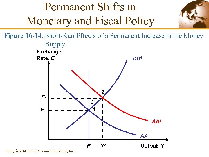
Permanent Shifts in Monetary and Fiscal Policy Figure 16 -14: Short-Run Effects of a Permanent Increase in the Money Supply Exchange Rate, E DD 1 2 E 2 3 1 E 1 AA 2 AA 1 Copyright © 2003 Pearson Education, Inc. Yf Y 2 Output, Y

Permanent Shifts in Monetary and Fiscal Policy § Adjustment to a Permanent Increase in the Money Supply • The permanent increase in the money supply raises output above its full-employment level. – As a result, the price level increases to bring the economy back to full employment. • Figure 16 -15 shows the adjustment back to full employment. Copyright © 2003 Pearson Education, Inc.

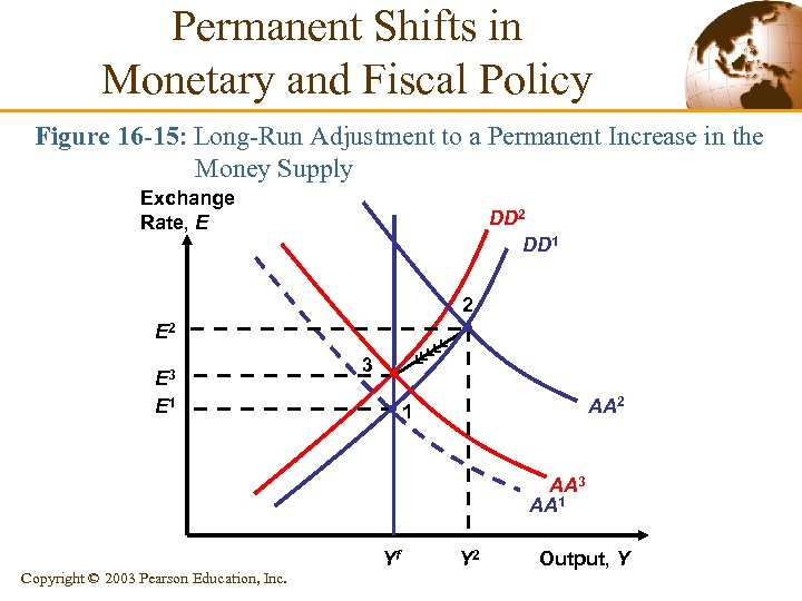
Permanent Shifts in Monetary and Fiscal Policy Figure 16 -15: Long-Run Adjustment to a Permanent Increase in the Money Supply Exchange Rate, E DD 2 DD 1 2 E 3 E 1 3 AA 2 1 AA 3 AA 1 Copyright © 2003 Pearson Education, Inc. Yf Y 2 Output, Y

Permanent Shifts in Monetary and Fiscal Policy § A Permanent Fiscal Expansion • A permanent fiscal expansion changes the long-run expected exchange rate. – If the economy starts at long-run equilibrium, a permanent change in fiscal policy has no effect on output. – It causes an immediate and permanent exchange rate jump that offsets exactly the fiscal policy’s direct effect on aggregate demand. Copyright © 2003 Pearson Education, Inc.

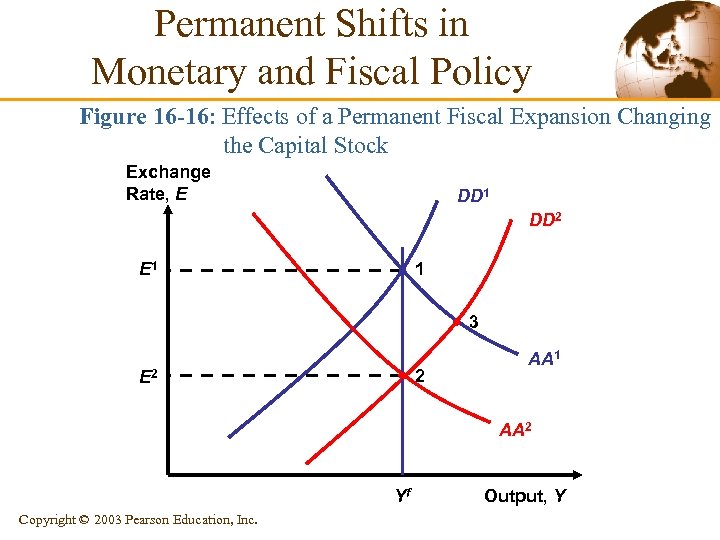
Permanent Shifts in Monetary and Fiscal Policy Figure 16 -16: Effects of a Permanent Fiscal Expansion Changing the Capital Stock Exchange Rate, E DD 1 DD 2 E 1 1 3 2 E 2 AA 1 AA 2 Yf Copyright © 2003 Pearson Education, Inc. Output, Y

Macroeconomic Policies and the Current Account § XX schedule • It shows combinations of the exchange rate and output • • at which the CA balance would be equal to some desired level. It slopes upward because a rise in output encourages spending on imports and thus worsens the current account (if it is not accompanied by a currency depreciation). It is flatter than DD. Copyright © 2003 Pearson Education, Inc.

Macroeconomic Policies and the Current Account • Monetary expansion causes the CA balance to increase • in the short run (point 2 in Figure 16 -17). Expansionary fiscal policy reduces the CA balance. – If it is temporary, the DD schedule shifts to the right (point 3 in Figure 16 -17). – If it is permanent, both AA and DD schedules shift (point 4 in Figure 16 -17). Copyright © 2003 Pearson Education, Inc.

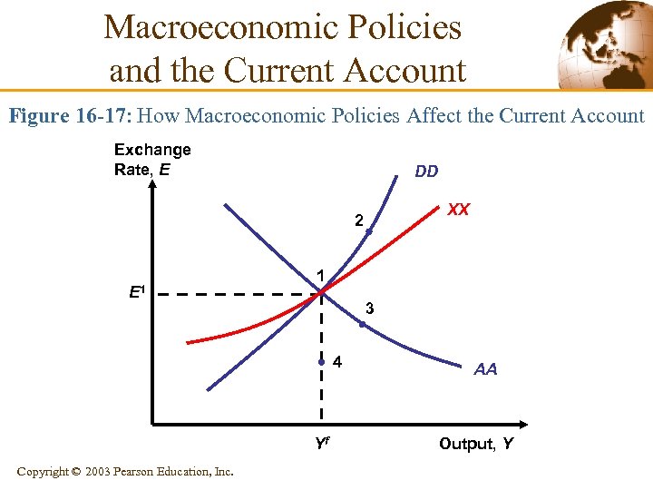
Macroeconomic Policies and the Current Account Figure 16 -17: How Macroeconomic Policies Affect the Current Account Exchange Rate, E DD XX 2 E 1 1 3 4 Yf Copyright © 2003 Pearson Education, Inc. AA Output, Y

Gradual Trade Flow Adjustment and Current Account Dynamics § The J-Curve • If imports and exports adjust gradually to real exchange rate changes, the CA may follow a J-curve pattern after a real currency depreciation, first worsening and then improving. – Currency depreciation may have a contractionary initial effect on output, and exchange rate overshooting will be amplified. • It describes the time lag with which a real currency depreciation improves the CA. Copyright © 2003 Pearson Education, Inc.

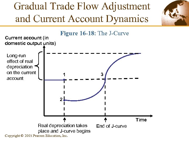
Gradual Trade Flow Adjustment and Current Account Dynamics Current account (in domestic output units) Figure 16 -18: The J-Curve Long-run effect of real depreciation on the current account 1 3 2 Time Real depreciation takes place and J-curve begins Copyright © 2003 Pearson Education, Inc. End of J-curve

Gradual Trade Flow Adjustment and Current Account Dynamics § Exchange Rate Pass-Through and Inflation • The CA in the DD-AA model has assumed that nominal • exchange rate changes cause proportional changes in the real exchange rates in the short run. Degree of Pass-through – It is the percentage by which import prices rise when the home currency depreciates by 1%. – In the DD-AA model, the degree of pass-through is 1. – Exchange rate pass-through can be incomplete because of international market segmentation. – Currency movements have less-than-proportional effects on the relative prices determining trade volumes. Copyright © 2003 Pearson Education, Inc.

Fixed versus Floating Exchange Rates § In the former model, exchange rates were considered § § as perfectly flexible. In reality, exchange rates are managed and rarely in a pure-floating system (Table 17 -1 in the textbook). The central bank can manage exchange rates using its foreign reserves. Copyright © 2003 Pearson Education, Inc.

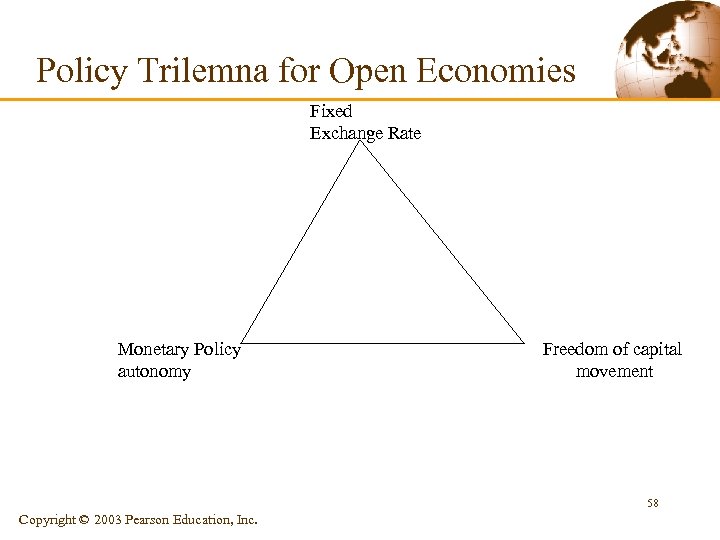
Fixed Exchange Rates § Monetary Policy Autonomy is lost (triangle), Fiscal § policy more efficient. Symetry: • Ex : USD and the Bretton Woods system, DM and the • european ER mechanism Support foreign shocks § Exchange Rates cannot adjust so there could be § persistent misalignments More investments and international trade Copyright © 2003 Pearson Education, Inc.

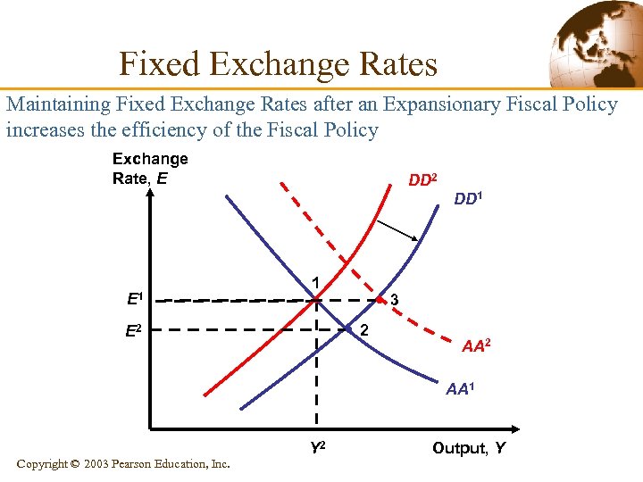
Fixed Exchange Rates Maintaining Fixed Exchange Rates after an Expansionary Fiscal Policy increases the efficiency of the Fiscal Policy Exchange Rate, E DD 2 DD 1 E 1 1 3 2 E 2 AA 1 Copyright © 2003 Pearson Education, Inc. Y 2 Output, Y

Policy Trilemna for Open Economies Fixed Exchange Rate Monetary Policy autonomy Freedom of capital

Floating Exchange Rates § Lack of Discipline (inflation, competitive § § depreciation…) More volatility that may dissuade investment and international trade No speculative pressure, exchange rates as automatic stabilizers (shocks easier to absorb, see the following figure). Copyright © 2003 Pearson Education, Inc.

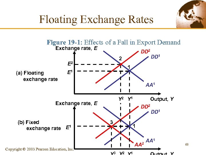
Floating Exchange Rates Figure 19 -1: Effects of a Fall in Export Demand Exchange rate, E DD 2 2 E 2 (a) Floating exchange rate 1 E 1 AA 1 Y 2 Y 1 Exchange rate, E (b) Fixed 1 exchange rate E Copyright © 2003 Pearson Education, Inc. DD 1 Output, Y DD 2 3 DD 1 1 AA 2 3 2 1 AA 1 60

Exchange rate crisis § The case of the european ER Mechanism • EMS (European Monetary System) fixed parities • • between european countries currency since 1979 1989 German reunification 1991 Perfect mobility of capital 1992 June, the Danish say « No » to the Maastricht Treaty, and France say « Yes » with only less than 51% 1992 -1993 Crisis Copyright © 2003 Pearson Education, Inc.

Exchange Rate Crisis § East Asian Crisis • Characteristics of Asian countries : high growth rate, • high degree of openess to the world market, low inflation rate, high saving rate but high investment rate (CA deficit). High profitability of investment opportunities, low uncertainty because of the stability Copyright © 2003 Pearson Education, Inc.

• Asian Weaknesses: – low productivity growth rate, growth due to a rise in inputs>diminishing returns – Banking regulation: no effective government supervision of banks, excessive lendings (bad loans) – Legal framework concerning bankruptcy • Starting point: – 1997, July, 2 devaluation of the Thai Baht – Contagion + economic slowdown of Japan -> East Asian countries could – Rise interest rates – Devaluate (rise in the domestic currency value of the debt) Copyright © 2003 Pearson Education, Inc.

Final Exam § The Final Exam covers all the course. § You have to read Mishkin’s textbook p. 469 -472 and § chapter 22 of the Krugman and Obstfeld’s textbook 2 hours, 6 questions among 7. Copyright © 2003 Pearson Education, Inc.