Financial Engineering Zvi Wiener mswiener mscc huji ac il

Financial Engineering Zvi Wiener mswiener@mscc. huji. ac. il tel: 02 -588 -3049 Zvi Wiener Cont. Time. Fin - 2 1

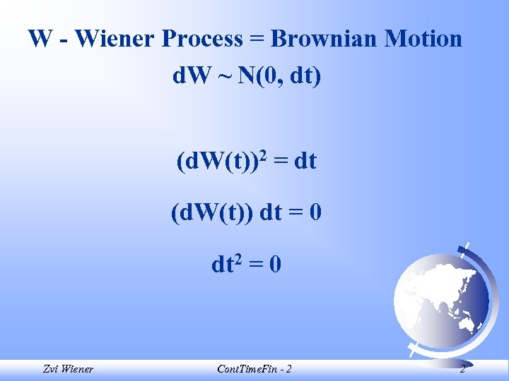W - Wiener Process = Brownian Motion d. W ~ N(0, dt) (d. W(t))2 = dt (d. W(t)) dt = 0 dt 2 = 0 Zvi Wiener Cont. Time. Fin - 2 2

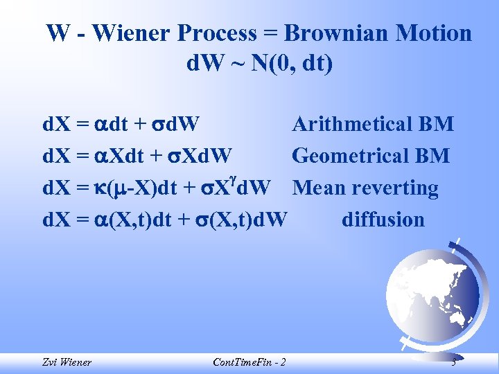W - Wiener Process = Brownian Motion d. W ~ N(0, dt) d. X = dt + d. W Arithmetical BM d. X = Xdt + Xd. W Geometrical BM d. X = ( -X)dt + X d. W Mean reverting d. X = (X, t)dt + (X, t)d. W diffusion Zvi Wiener Cont. Time. Fin - 2 3

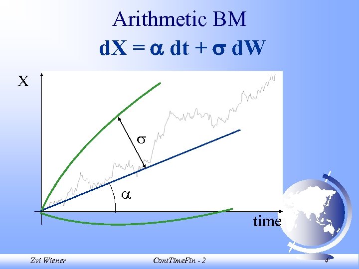Arithmetic BM d. X = dt + d. W X time Zvi Wiener Cont. Time. Fin - 2 4

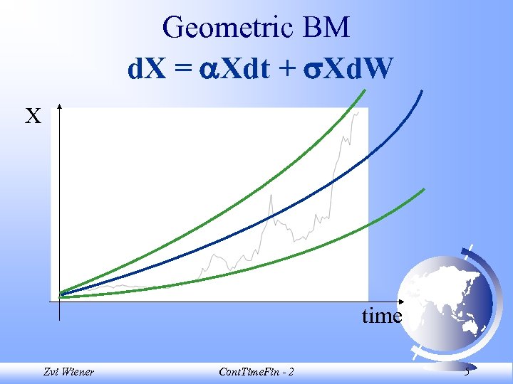Geometric BM d. X = Xdt + Xd. W X time Zvi Wiener Cont. Time. Fin - 2 5

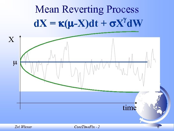Mean Reverting Process d. X = ( -X)dt + X d. W X time Zvi Wiener Cont. Time. Fin - 2 6

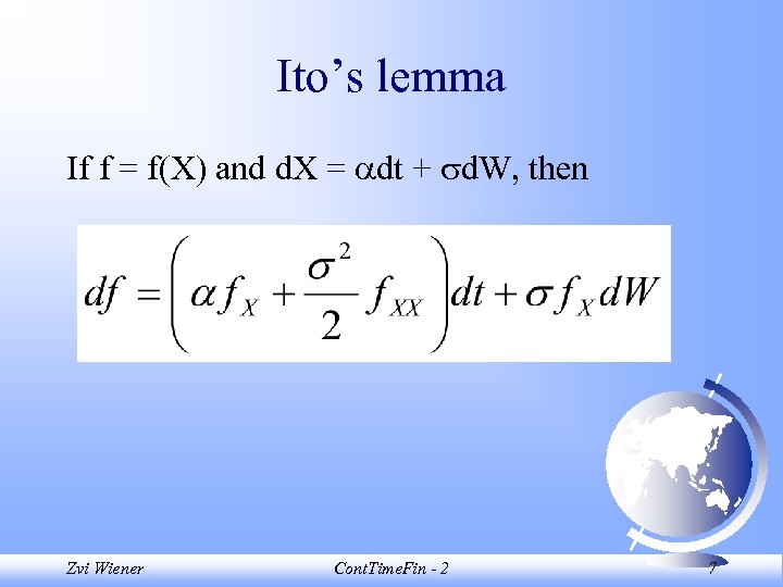Ito’s lemma If f = f(X) and d. X = dt + d. W, then Zvi Wiener Cont. Time. Fin - 2 7

Multivariate Ito’s Lemma Introduce a second variable Y to the system that follows a diffusion d. X = (X, Y, t)dt + (X, Y, t)d. W d. Y = (X, Y, t)dt + (X, Y, t)d. Z where Z is another standard Wiener process. We define d. Zd. W = dt as the correlation between the two processes. Zvi Wiener Cont. Time. Fin - 2 8

Multivariate Ito’s Lemma It can be shown that E[d. Zd. W] = dt (d. Zd. W)2 = 0 Probabilistically d. Z can be projected on d. W d. Z = d. W + (1 - 2)1/2 de where de is a standard Wiener process uncorrelated with d. W, de d. W = 0 Zvi Wiener Cont. Time. Fin - 2 9

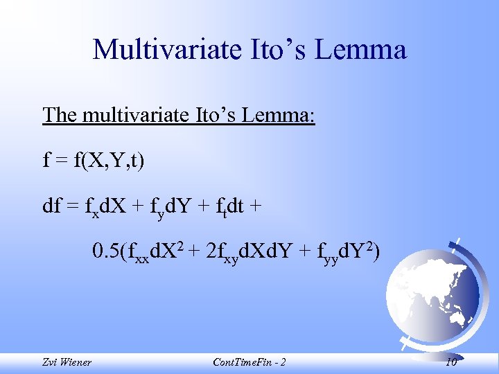Multivariate Ito’s Lemma The multivariate Ito’s Lemma: f = f(X, Y, t) df = fxd. X + fyd. Y + ftdt + 0. 5(fxxd. X 2 + 2 fxyd. Xd. Y + fyyd. Y 2) Zvi Wiener Cont. Time. Fin - 2 10

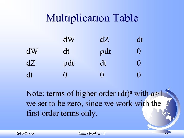Multiplication Table d. W d. Z dt d. W dt dt 0 d. Z dt dt 0 0 0 Note: terms of higher order (dt)a with a>1 we set to be zero, since we work with the first order terms only. Zvi Wiener Cont. Time. Fin - 2 11

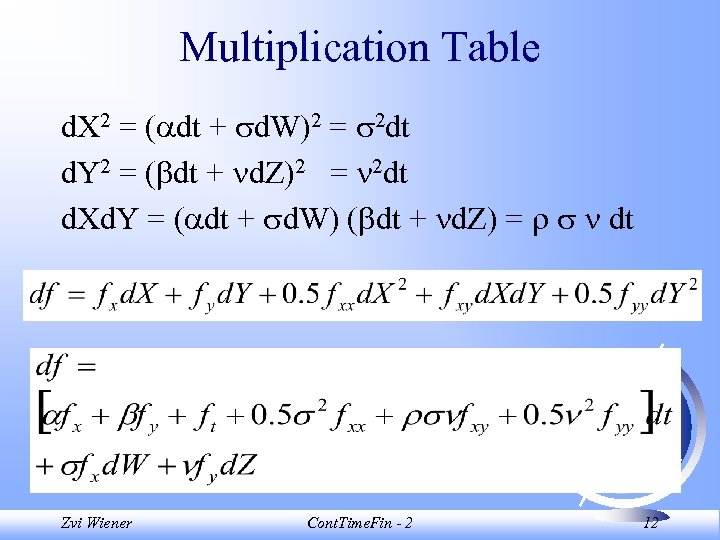Multiplication Table d. X 2 = ( dt + d. W)2 = 2 dt d. Y 2 = ( dt + d. Z)2 = 2 dt d. Xd. Y = ( dt + d. W) ( dt + d. Z) = dt Zvi Wiener Cont. Time. Fin - 2 12

Jump Processes Diffusion processes are continuous. In order to include jumps we use Poisson processes. Define q(t) such that q(0) = 0 and is constant until a Poisson event occurs. When there is a Poisson event value of q increases by 1. Zvi Wiener Cont. Time. Fin - 2 13

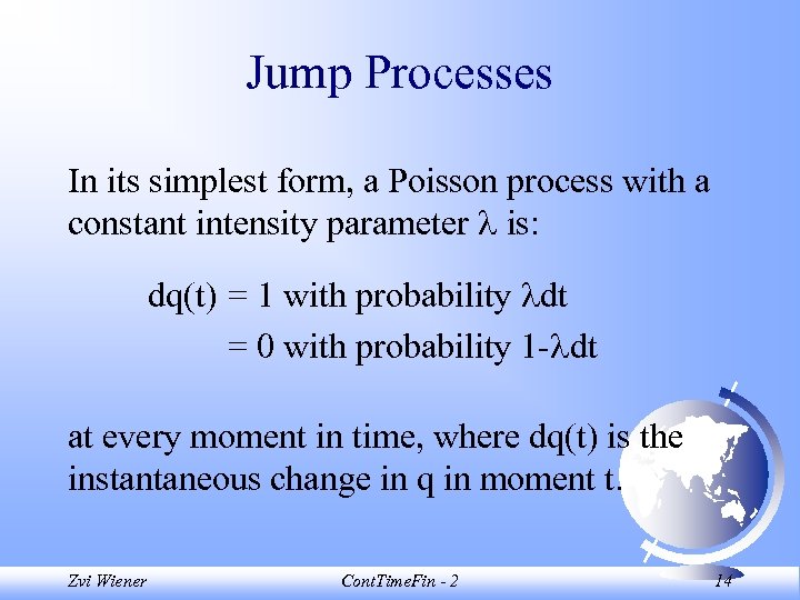Jump Processes In its simplest form, a Poisson process with a constant intensity parameter is: dq(t) = 1 with probability dt = 0 with probability 1 - dt at every moment in time, where dq(t) is the instantaneous change in q in moment t. Zvi Wiener Cont. Time. Fin - 2 14

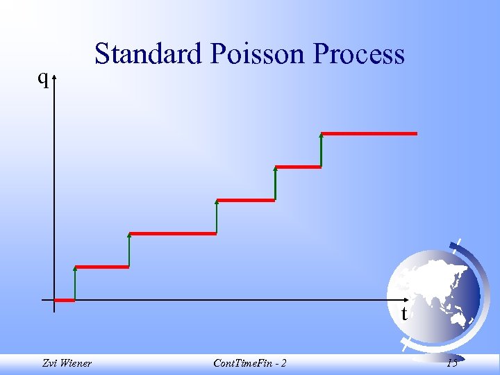q Standard Poisson Process t Zvi Wiener Cont. Time. Fin - 2 15

Standard Poisson Process jump[lam_, dt_]: =If[ Random[ ] < lam*dt, 1, 0]; tt = Nest. List[(# + jump[0. 5, 0. 1])&, 0, 300]; List. Plot[tt, Plot. Joined->True]; Zvi Wiener Cont. Time. Fin - 2 16

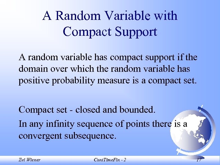A Random Variable with Compact Support A random variable has compact support if the domain over which the random variable has positive probability measure is a compact set. Compact set - closed and bounded. In any infinity sequence of points there is a convergent subsequence. Zvi Wiener Cont. Time. Fin - 2 17

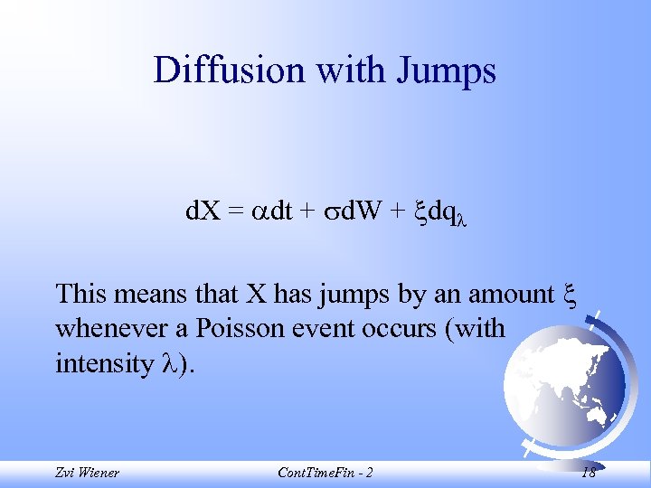Diffusion with Jumps d. X = dt + d. W + dq This means that X has jumps by an amount whenever a Poisson event occurs (with intensity ). Zvi Wiener Cont. Time. Fin - 2 18

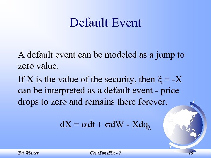Default Event A default event can be modeled as a jump to zero value. If X is the value of the security, then = -X can be interpreted as a default event - price drops to zero and remains there forever. d. X = dt + d. W - Xdq Zvi Wiener Cont. Time. Fin - 2 19

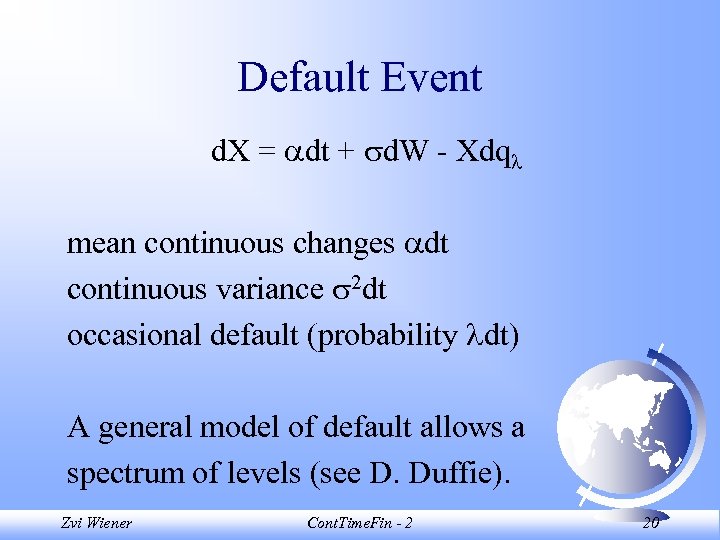Default Event d. X = dt + d. W - Xdq mean continuous changes dt continuous variance 2 dt occasional default (probability dt) A general model of default allows a spectrum of levels (see D. Duffie). Zvi Wiener Cont. Time. Fin - 2 20

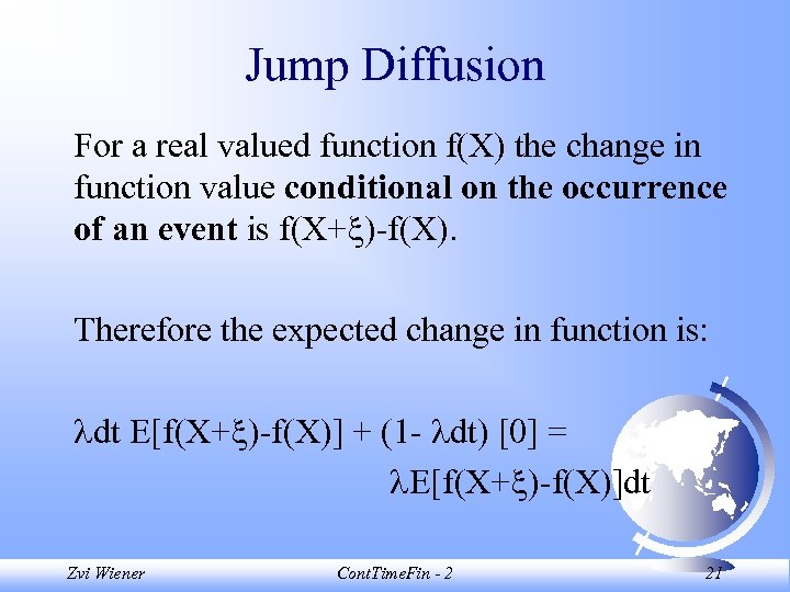Jump Diffusion For a real valued function f(X) the change in function value conditional on the occurrence of an event is f(X+ )-f(X). Therefore the expected change in function is: dt E[f(X+ )-f(X)] + (1 - dt) [0] = E[f(X+ )-f(X)]dt Zvi Wiener Cont. Time. Fin - 2 21

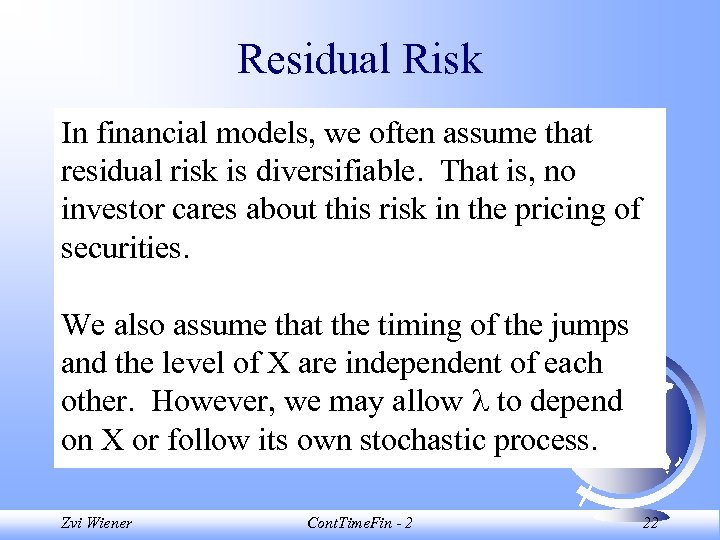Residual Risk In financial models, we often assume that residual risk is diversifiable. That is, no investor cares about this risk in the pricing of securities. We also assume that the timing of the jumps and the level of X are independent of each other. However, we may allow to depend on X or follow its own stochastic process. Zvi Wiener Cont. Time. Fin - 2 22

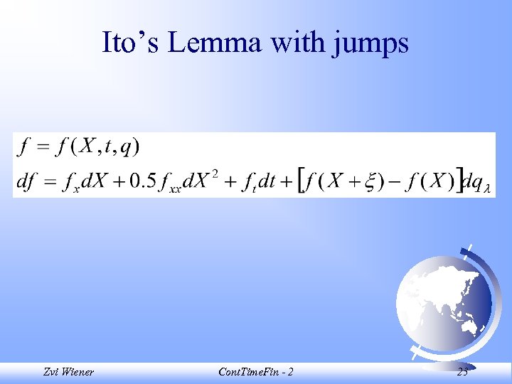Ito’s Lemma with jumps Zvi Wiener Cont. Time. Fin - 2 23

Financial Applications A Suppose that a security with value V guarantees $1 dt every instant of time forever. This is the continuous time equivalent of a risk-free perpetuity of $1. If the risk-free interest rate is constant r, what is the (discounted) value of the security? Zvi Wiener Cont. Time. Fin - 2 24

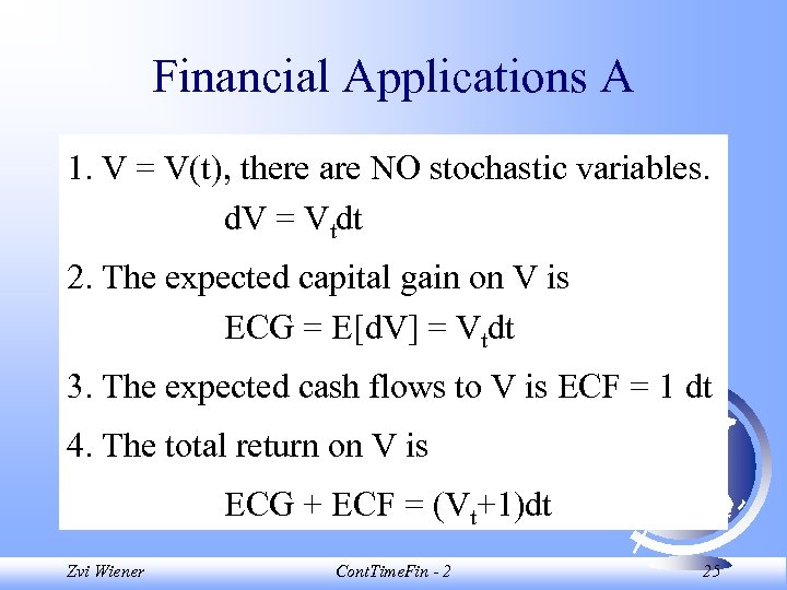Financial Applications A 1. V = V(t), there are NO stochastic variables. d. V = Vtdt 2. The expected capital gain on V is ECG = E[d. V] = Vtdt 3. The expected cash flows to V is ECF = 1 dt 4. The total return on V is ECG + ECF = (Vt+1)dt Zvi Wiener Cont. Time. Fin - 2 25

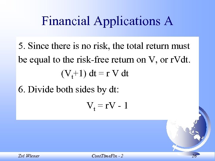Financial Applications A 5. Since there is no risk, the total return must be equal to the risk-free return on V, or r. Vdt. (Vt+1) dt = r V dt 6. Divide both sides by dt: Vt = r. V - 1 Zvi Wiener Cont. Time. Fin - 2 26

Financial Applications A Vt = r. V - 1 DSolve[ V'[t]==r*V[t]-1, V[t], t ] V(t) = c Exp[r t] + 1/r given V(0) one can find c Zvi Wiener Cont. Time. Fin - 2 27

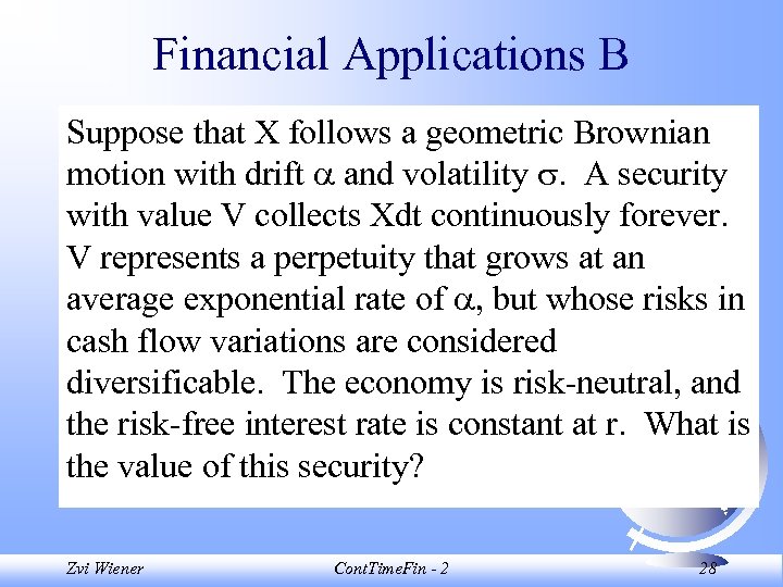Financial Applications B Suppose that X follows a geometric Brownian motion with drift and volatility . A security with value V collects Xdt continuously forever. V represents a perpetuity that grows at an average exponential rate of , but whose risks in cash flow variations are considered diversificable. The economy is risk-neutral, and the risk-free interest rate is constant at r. What is the value of this security? Zvi Wiener Cont. Time. Fin - 2 28

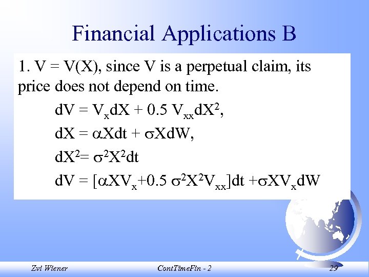Financial Applications B 1. V = V(X), since V is a perpetual claim, its price does not depend on time. d. V = Vxd. X + 0. 5 Vxxd. X 2, d. X = Xdt + Xd. W, d. X 2= 2 X 2 dt d. V = [ XVx+0. 5 2 X 2 Vxx]dt + XVxd. W Zvi Wiener Cont. Time. Fin - 2 29

Financial Applications B 2. The expected capital gain: ECG = E[d. V] = [ XVx+0. 5 2 X 2 Vxx]dt since E[d. W] = 0 3. The Expected cash flow: ECF = X dt Zvi Wiener Cont. Time. Fin - 2 30

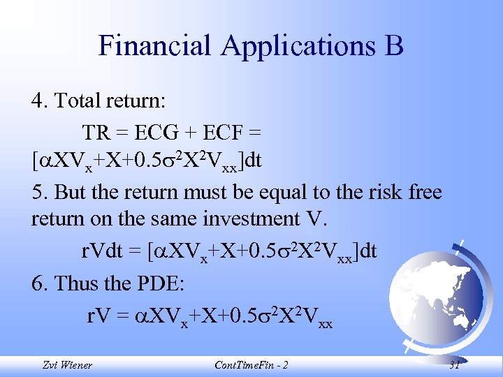Financial Applications B 4. Total return: TR = ECG + ECF = [ XVx+X+0. 5 2 X 2 Vxx]dt 5. But the return must be equal to the risk free return on the same investment V. r. Vdt = [ XVx+X+0. 5 2 X 2 Vxx]dt 6. Thus the PDE: r. V = XVx+X+0. 5 2 X 2 Vxx Zvi Wiener Cont. Time. Fin - 2 31

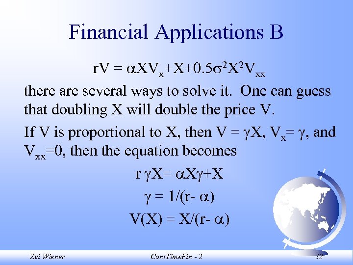Financial Applications B r. V = XVx+X+0. 5 2 X 2 Vxx there are several ways to solve it. One can guess that doubling X will double the price V. If V is proportional to X, then V = X, Vx= , and Vxx=0, then the equation becomes r X= X +X = 1/(r- ) V(X) = X/(r- ) Zvi Wiener Cont. Time. Fin - 2 32

Financial Applications C Modify example B to provide for a sudden possible drop to zero in the value of V. If a Poisson event occurs, one gives up V in exchange for nothing. The gain is zero and the loss is V, so the change in the value of V is 0 -V, or -V. The possibility of this jump in any instant is dt. Zvi Wiener Cont. Time. Fin - 2 33

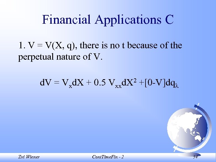Financial Applications C 1. V = V(X, q), there is no t because of the perpetual nature of V. d. V = Vxd. X + 0. 5 Vxxd. X 2 +[0 -V]dq Zvi Wiener Cont. Time. Fin - 2 34

Financial Applications C 2. Expected Capital Gain: ECG = E[d. V] = [ XVx+0. 5 2 X 2 Vxx- V]dt 3. Expected Cash Flow: ECF = Xdt Zvi Wiener Cont. Time. Fin - 2 35

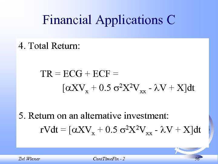Financial Applications C 4. Total Return: TR = ECG + ECF = [ XVx + 0. 5 2 X 2 Vxx - V + X]dt 5. Return on an alternative investment: r. Vdt = [ XVx + 0. 5 2 X 2 Vxx - V + X]dt Zvi Wiener Cont. Time. Fin - 2 36

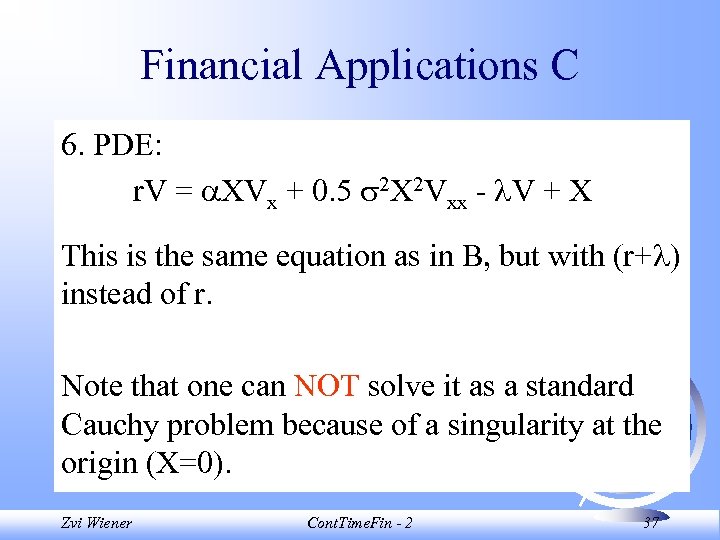Financial Applications C 6. PDE: r. V = XVx + 0. 5 2 X 2 Vxx - V + X This is the same equation as in B, but with (r+ ) instead of r. Note that one can NOT solve it as a standard Cauchy problem because of a singularity at the origin (X=0). Zvi Wiener Cont. Time. Fin - 2 37

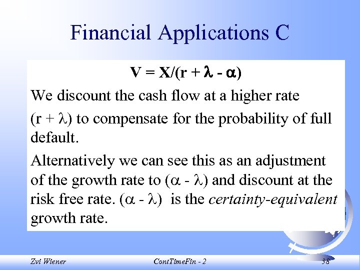Financial Applications C V = X/(r + - ) We discount the cash flow at a higher rate (r + ) to compensate for the probability of full default. Alternatively we can see this as an adjustment of the growth rate to ( - ) and discount at the risk free rate. ( - ) is the certainty-equivalent growth rate. Zvi Wiener Cont. Time. Fin - 2 38

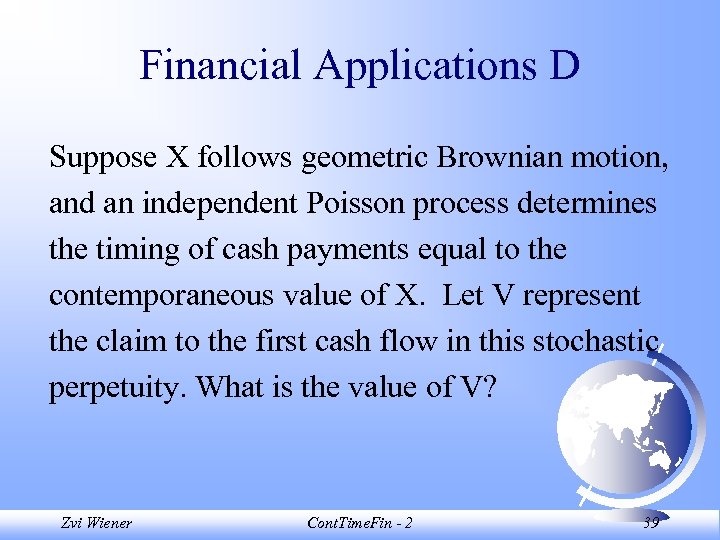Financial Applications D Suppose X follows geometric Brownian motion, and an independent Poisson process determines the timing of cash payments equal to the contemporaneous value of X. Let V represent the claim to the first cash flow in this stochastic perpetuity. What is the value of V? Zvi Wiener Cont. Time. Fin - 2 39

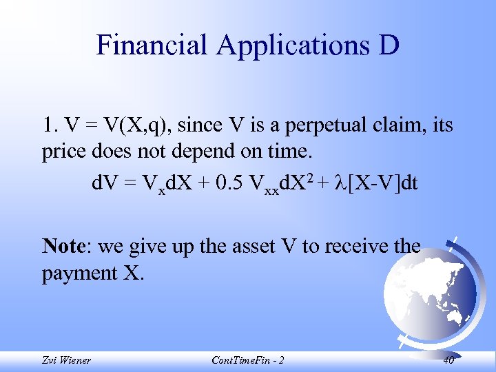Financial Applications D 1. V = V(X, q), since V is a perpetual claim, its price does not depend on time. d. V = Vxd. X + 0. 5 Vxxd. X 2 + [X-V]dt Note: we give up the asset V to receive the payment X. Zvi Wiener Cont. Time. Fin - 2 40

Financial Applications D 2. The expected capital gain: ECG = E[d. V] = [ XVx+0. 5 2 X 2 Vxx+ (X-V)]dt 3. The Expected cash flow: ECF = 0 There are no continuous cash payments. Zvi Wiener Cont. Time. Fin - 2 41

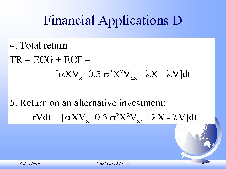Financial Applications D 4. Total return TR = ECG + ECF = [ XVx+0. 5 2 X 2 Vxx+ X - V]dt 5. Return on an alternative investment: r. Vdt = [ XVx+0. 5 2 X 2 Vxx+ X - V]dt Zvi Wiener Cont. Time. Fin - 2 42

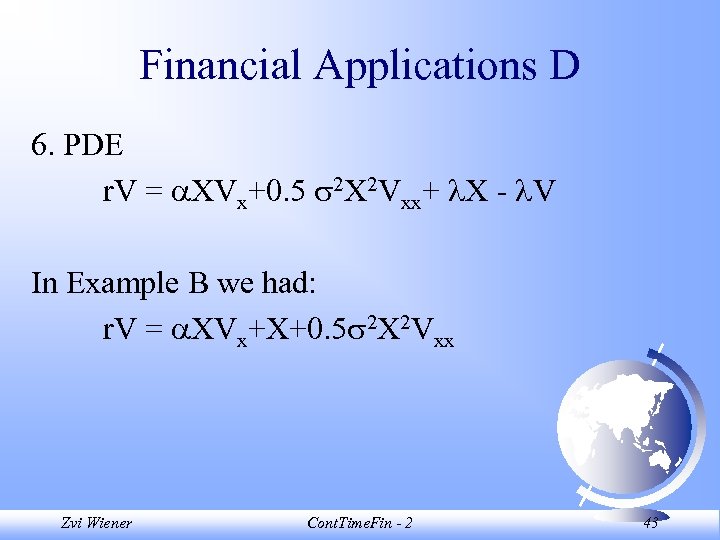Financial Applications D 6. PDE r. V = XVx+0. 5 2 X 2 Vxx+ X - V In Example B we had: r. V = XVx+X+0. 5 2 X 2 Vxx Zvi Wiener Cont. Time. Fin - 2 43

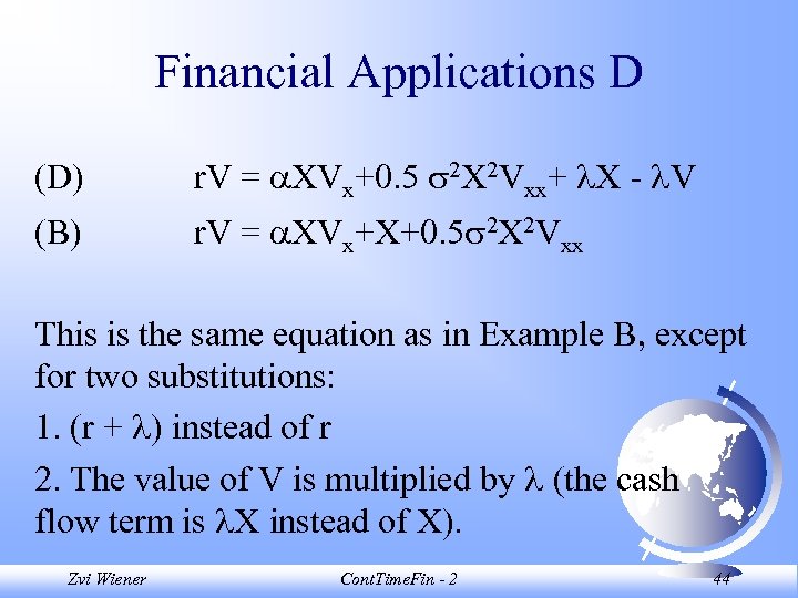Financial Applications D (D) r. V = XVx+0. 5 2 X 2 Vxx+ X - V (B) r. V = XVx+X+0. 5 2 X 2 Vxx This is the same equation as in Example B, except for two substitutions: 1. (r + ) instead of r 2. The value of V is multiplied by (the cash flow term is X instead of X). Zvi Wiener Cont. Time. Fin - 2 44

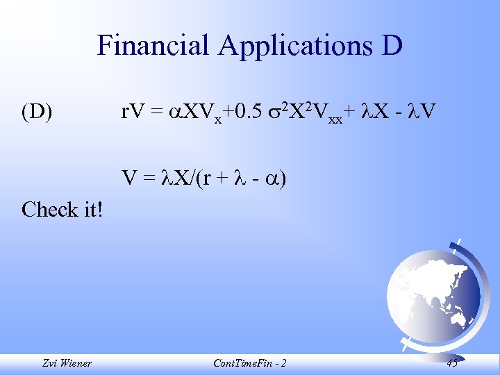Financial Applications D (D) r. V = XVx+0. 5 2 X 2 Vxx+ X - V V = X/(r + - ) Check it! Zvi Wiener Cont. Time. Fin - 2 45

Conclusions We have studied Present Value (PV) calculations in continuous time settings. We have received ODE, since all our models were perpetual (no explicit time dependence). Zvi Wiener Cont. Time. Fin - 2 46

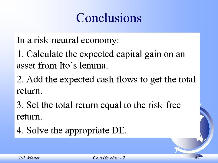Conclusions In a risk-neutral economy: 1. Calculate the expected capital gain on an asset from Ito’s lemma. 2. Add the expected cash flows to get the total return. 3. Set the total return equal to the risk-free return. 4. Solve the appropriate DE. Zvi Wiener Cont. Time. Fin - 2 47

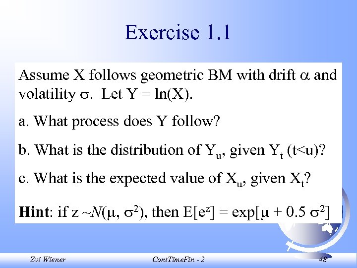Exercise 1. 1 Assume X follows geometric BM with drift and volatility . Let Y = ln(X). a. What process does Y follow? b. What is the distribution of Yu, given Yt (t

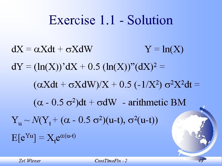Exercise 1. 1 - Solution d. X = Xdt + Xd. W Y = ln(X) d. Y = (ln(X))’d. X + 0. 5 (ln(X))”(d. X)2 = ( Xdt + Xd. W)/X + 0. 5 (-1/X 2) 2 X 2 dt = ( - 0. 5 2)dt + d. W - arithmetic BM Yu ~ N(Yt + ( - 0. 5 2)(u-t), 2(u-t)) E[e. Yu] = Xte (u-t) Zvi Wiener Cont. Time. Fin - 2 49

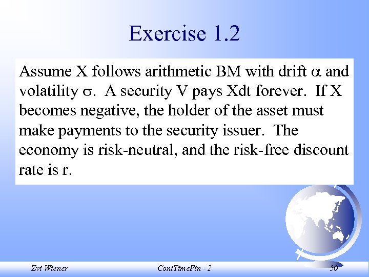Exercise 1. 2 Assume X follows arithmetic BM with drift and volatility . A security V pays Xdt forever. If X becomes negative, the holder of the asset must make payments to the security issuer. The economy is risk-neutral, and the risk-free discount rate is r. Zvi Wiener Cont. Time. Fin - 2 50

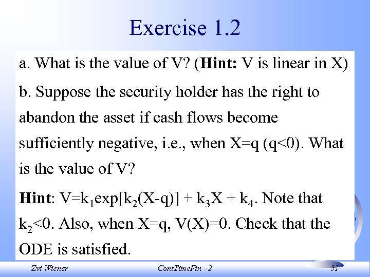Exercise 1. 2 a. What is the value of V? (Hint: V is linear in X) b. Suppose the security holder has the right to abandon the asset if cash flows become sufficiently negative, i. e. , when X=q (q<0). What is the value of V? Hint: V=k 1 exp[k 2(X-q)] + k 3 X + k 4. Note that k 2<0. Also, when X=q, V(X)=0. Check that the ODE is satisfied. Zvi Wiener Cont. Time. Fin - 2 51

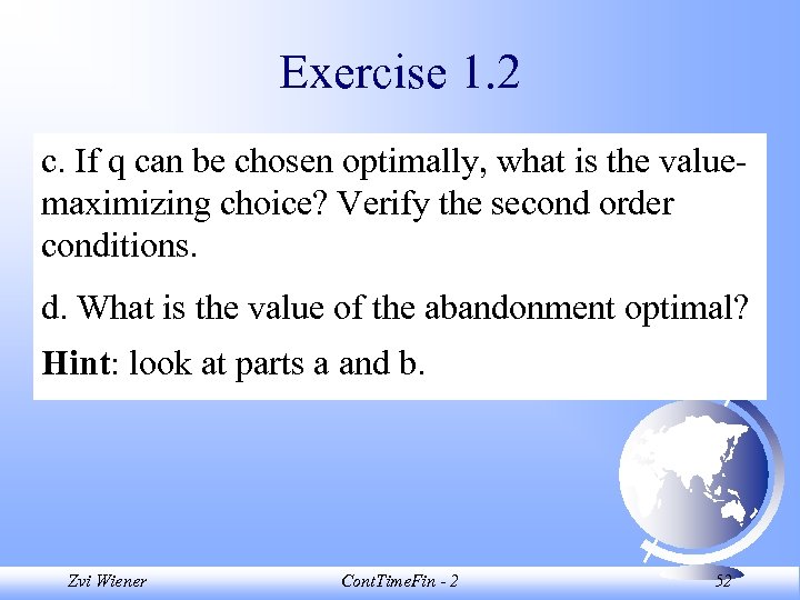Exercise 1. 2 c. If q can be chosen optimally, what is the valuemaximizing choice? Verify the second order conditions. d. What is the value of the abandonment optimal? Hint: look at parts a and b. Zvi Wiener Cont. Time. Fin - 2 52

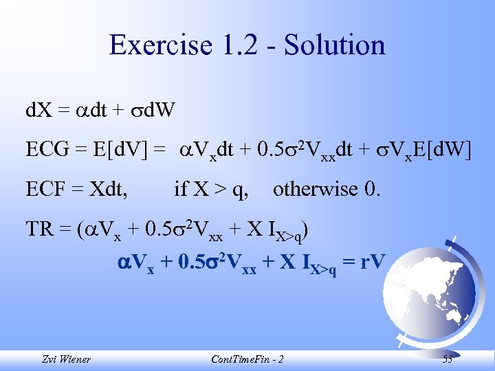Exercise 1. 2 - Solution d. X = dt + d. W ECG = E[d. V] = Vxdt + 0. 5 2 Vxxdt + Vx. E[d. W] ECF = Xdt, if X > q, otherwise 0. TR = ( Vx + 0. 5 2 Vxx + X IX>q) Vx + 0. 5 2 Vxx + X IX>q = r. V Zvi Wiener Cont. Time. Fin - 2 53

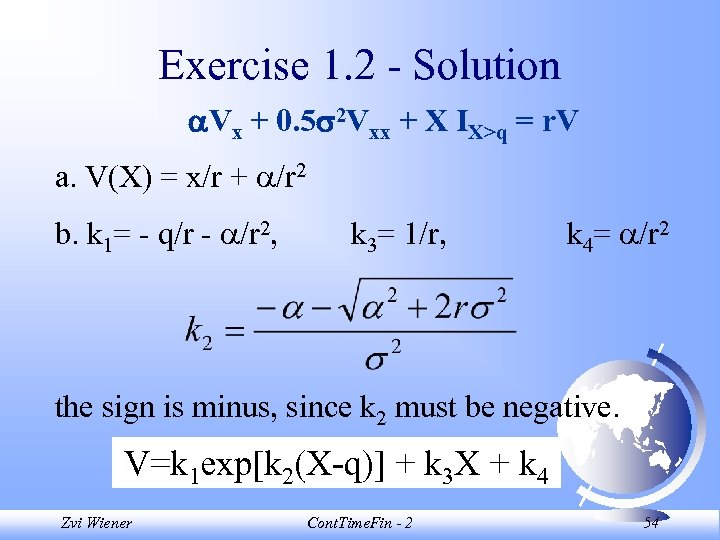Exercise 1. 2 - Solution Vx + 0. 5 2 Vxx + X IX>q = r. V a. V(X) = x/r + /r 2 b. k 1= - q/r - /r 2, k 3= 1/r, k 4= /r 2 the sign is minus, since k 2 must be negative. V=k 1 exp[k 2(X-q)] + k 3 X + k 4 Zvi Wiener Cont. Time. Fin - 2 54

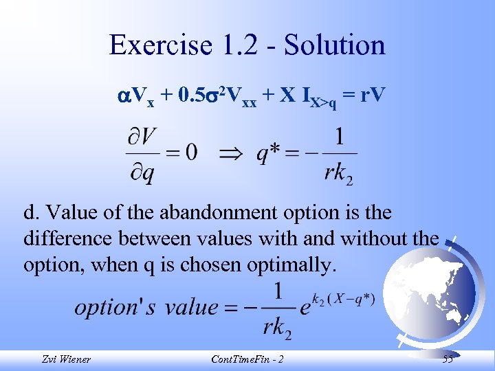Exercise 1. 2 - Solution Vx + 0. 5 2 Vxx + X IX>q = r. V d. Value of the abandonment option is the difference between values with and without the option, when q is chosen optimally. Zvi Wiener Cont. Time. Fin - 2 55

Exercise 1. 3 Assume that X follows geometric BM, with drift and volatility . The economy is risk-neutral, and the risk-free discount rate is r. A machine prints a certificate worth X(t) at random times t generated by a Poisson arrival process with intensity . a. What is the value of this machine? b. What is the value of a contingent claim to the first certificate printed by the machine? Zvi Wiener Cont. Time. Fin - 2 56

Exercise 1. 3 c. Assume Y follows geometric BM with drift and volatility . The correlation between X and Y is 0. What is the value of a certificate produced by X, if it lets its bearer (only) have X certificates printed by machine Y (worth Y at the time of printing)? Y prints at the same average rate, and the number of certificates is determined by the first arrival time. Zvi Wiener Cont. Time. Fin - 2 57

Exercise 1. 3 - Solution a. d. X = Xdt + Xd. W ECG = E[d. V] = XVxdt + 0. 5 2 X 2 Vxxdt ECF = Xdt TR = ( XVx + 0. 5 X 2 2 Vxx + X)dt XVx + 0. 5 X 2 2 Vxx + X = r. V V(X)= X/(r - ) Zvi Wiener Cont. Time. Fin - 2 58

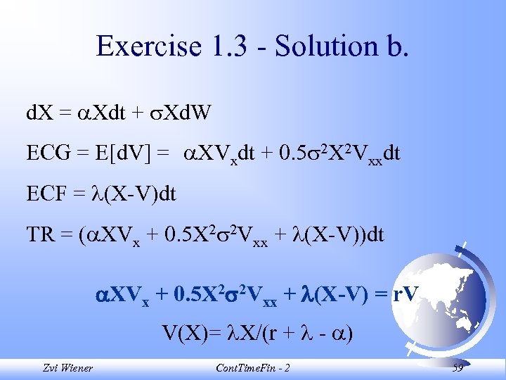Exercise 1. 3 - Solution b. d. X = Xdt + Xd. W ECG = E[d. V] = XVxdt + 0. 5 2 X 2 Vxxdt ECF = (X-V)dt TR = ( XVx + 0. 5 X 2 2 Vxx + (X-V))dt XVx + 0. 5 X 2 2 Vxx + (X-V) = r. V V(X)= X/(r + - ) Zvi Wiener Cont. Time. Fin - 2 59

Exercise 1. 4 A low-risk health insurance policy holder realizes medical losses at random times according to a Poisson arrival process. The level of the loss is given by X, a process which follows GBM with drift and volatility . The economy is riskneutral, and the risk-free discount rate is r. Medical expenses occur at a rate dt. There is an additional possibility that the claimant will suddenly become a high-risk claimant. Zvi Wiener Cont. Time. Fin - 2 60

Exercise 1. 4 High-risk claimants experience the same possible losses X, but at a higher frequency dt. The timing of the switch from a low-risk to a high-risk is governed by a Poisson process with intensity parameter . a. If the policy holder stays low-risk forever, what is the value of the policy today? b. What is the value of a high-risk policy today? c. What is the value of a low-risk policy today? Zvi Wiener Cont. Time. Fin - 2 61

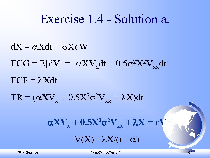Exercise 1. 4 - Solution a. d. X = Xdt + Xd. W ECG = E[d. V] = XVxdt + 0. 5 2 X 2 Vxxdt ECF = Xdt TR = ( XVx + 0. 5 X 2 2 Vxx + X)dt XVx + 0. 5 X 2 2 Vxx + X = r. V V(X)= X/(r - ) Zvi Wiener Cont. Time. Fin - 2 62

Exercise 1. 4 - Solution b. d. X = Xdt + Xd. W ECG = E[d. V] = XVxdt + 0. 5 2 X 2 Vxxdt ECF = Xdt TR = ( XVx + 0. 5 X 2 2 Vxx + X)dt XVx + 0. 5 X 2 2 Vxx + X = r. V V(X)= X/(r - ) Zvi Wiener Cont. Time. Fin - 2 63

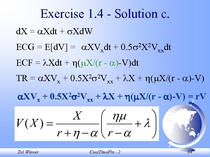Exercise 1. 4 - Solution c. d. X = Xdt + Xd. W ECG = E[d. V] = XVxdt + 0. 5 2 X 2 Vxxdt ECF = Xdt + ( X/(r - )-V)dt TR = XVx + 0. 5 X 2 2 Vxx + X + ( X/(r - )-V) = r. V Zvi Wiener Cont. Time. Fin - 2 64

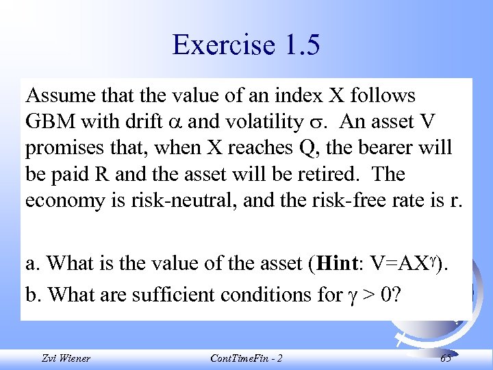Exercise 1. 5 Assume that the value of an index X follows GBM with drift and volatility . An asset V promises that, when X reaches Q, the bearer will be paid R and the asset will be retired. The economy is risk-neutral, and the risk-free rate is r. a. What is the value of the asset (Hint: V=AX ). b. What are sufficient conditions for > 0? Zvi Wiener Cont. Time. Fin - 2 65

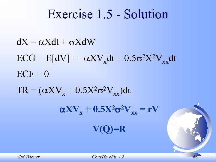Exercise 1. 5 - Solution d. X = Xdt + Xd. W ECG = E[d. V] = XVxdt + 0. 5 2 X 2 Vxxdt ECF = 0 TR = ( XVx + 0. 5 X 2 2 Vxx)dt XVx + 0. 5 X 2 2 Vxx = r. V V(Q)=R Zvi Wiener Cont. Time. Fin - 2 66

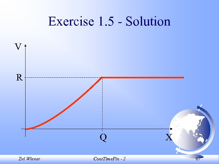Exercise 1. 5 - Solution V R Q Zvi Wiener Cont. Time. Fin - 2 X 67

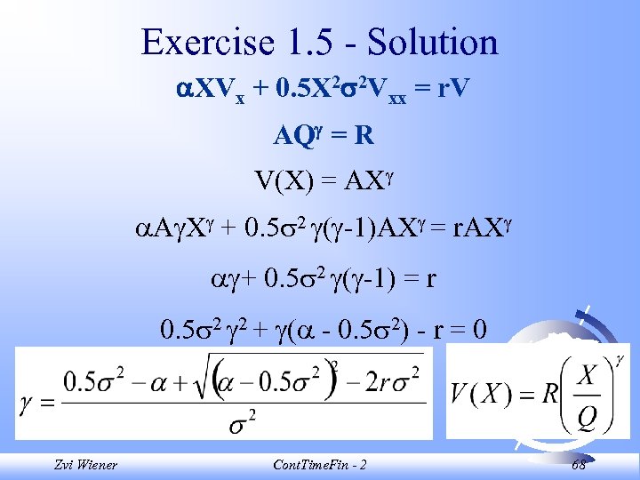Exercise 1. 5 - Solution XVx + 0. 5 X 2 2 Vxx = r. V AQ = R V(X) = AX A X + 0. 5 2 ( -1)AX = r. AX + 0. 5 2 ( -1) = r 0. 5 2 2 + ( - 0. 5 2) - r = 0 Zvi Wiener Cont. Time. Fin - 2 68

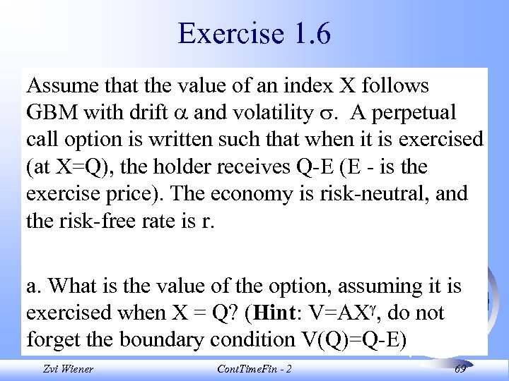Exercise 1. 6 Assume that the value of an index X follows GBM with drift and volatility . A perpetual call option is written such that when it is exercised (at X=Q), the holder receives Q-E (E - is the exercise price). The economy is risk-neutral, and the risk-free rate is r. a. What is the value of the option, assuming it is exercised when X = Q? (Hint: V=AX , do not forget the boundary condition V(Q)=Q-E) Zvi Wiener Cont. Time. Fin - 2 69

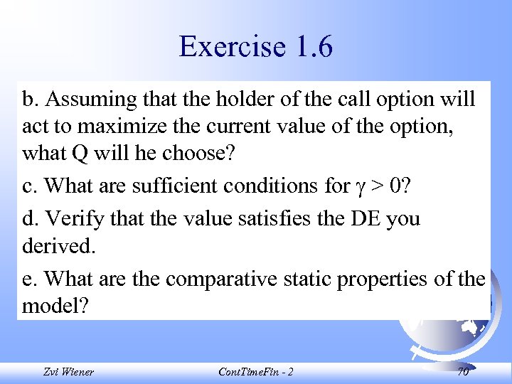Exercise 1. 6 b. Assuming that the holder of the call option will act to maximize the current value of the option, what Q will he choose? c. What are sufficient conditions for > 0? d. Verify that the value satisfies the DE you derived. e. What are the comparative static properties of the model? Zvi Wiener Cont. Time. Fin - 2 70

Exercise 1. 6 - Solution a. d. X = Xdt + Xd. W ECG = E[d. V] = XVxdt + 0. 5 2 X 2 Vxxdt ECF = 0 TR = ( XVx + 0. 5 X 2 2 Vxx)dt XVx + 0. 5 X 2 2 Vxx = r. V V(Q)=Q-E Zvi Wiener Cont. Time. Fin - 2 71

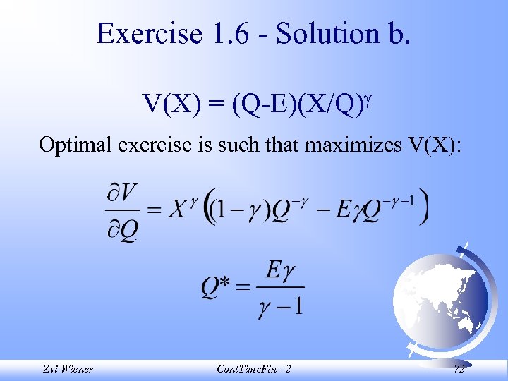Exercise 1. 6 - Solution b. V(X) = (Q-E)(X/Q) Optimal exercise is such that maximizes V(X): Zvi Wiener Cont. Time. Fin - 2 72

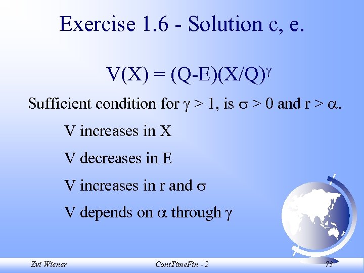Exercise 1. 6 - Solution c, e. V(X) = (Q-E)(X/Q) Sufficient condition for > 1, is > 0 and r > . V increases in X V decreases in E V increases in r and V depends on through Zvi Wiener Cont. Time. Fin - 2 73

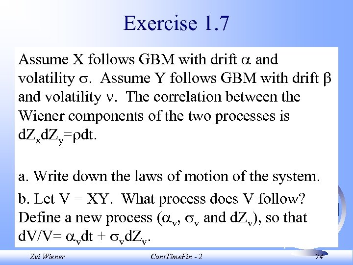Exercise 1. 7 Assume X follows GBM with drift and volatility . Assume Y follows GBM with drift and volatility . The correlation between the Wiener components of the two processes is d. Zxd. Zy= dt. a. Write down the laws of motion of the system. b. Let V = XY. What process does V follow? Define a new process ( v, v and d. Zv), so that d. V/V= vdt + vd. Zvi Wiener Cont. Time. Fin - 2 74

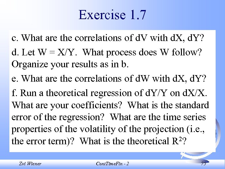Exercise 1. 7 c. What are the correlations of d. V with d. X, d. Y? d. Let W = X/Y. What process does W follow? Organize your results as in b. e. What are the correlations of d. W with d. X, d. Y? f. Run a theoretical regression of d. Y/Y on d. X/X. What are your coefficients? What is the standard error of the regression? What are the time series properties of the volatility of the projection (i. e. , the error term)? What is theoretical R 2? Zvi Wiener Cont. Time. Fin - 2 75

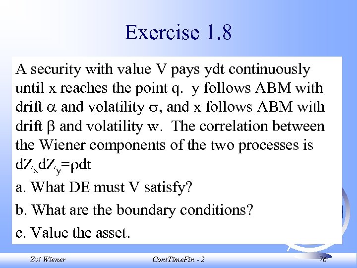Exercise 1. 8 A security with value V pays ydt continuously until x reaches the point q. y follows ABM with drift and volatility , and x follows ABM with drift and volatility w. The correlation between the Wiener components of the two processes is d. Zxd. Zy= dt a. What DE must V satisfy? b. What are the boundary conditions? c. Value the asset. Zvi Wiener Cont. Time. Fin - 2 76

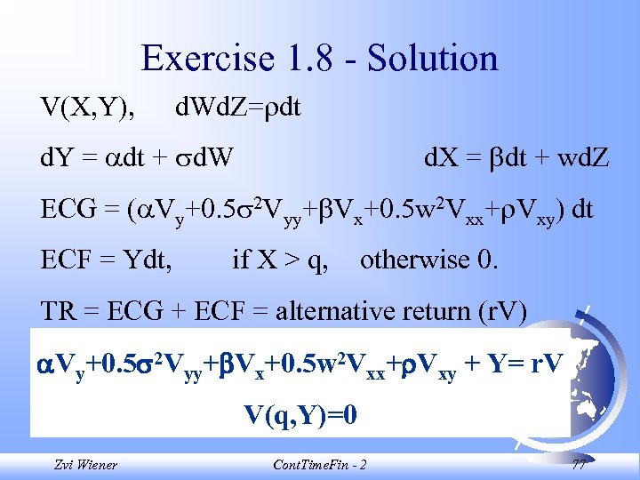Exercise 1. 8 - Solution V(X, Y), d. Wd. Z= dt d. Y = dt + d. W d. X = dt + wd. Z ECG = ( Vy+0. 5 2 Vyy+ Vx+0. 5 w 2 Vxx+ Vxy) dt ECF = Ydt, if X > q, otherwise 0. TR = ECG + ECF = alternative return (r. V) Vy+0. 5 2 Vyy+ Vx+0. 5 w 2 Vxx+ Vxy + Y= r. V V(q, Y)=0 Zvi Wiener Cont. Time. Fin - 2 77

Exercise 1. 9 A firm earns Xdt continuously, where X follows ABM with drift and volatility . This is the only asset of the firm. If X becomes negative, then the firm must decide whether to honor its obligations or abandon its operations. We assume it is optimal to abandon operations when earnings fall below a constant level q. The firm wishes to sell contingent claims against its earnings. Zvi Wiener Cont. Time. Fin - 2 78

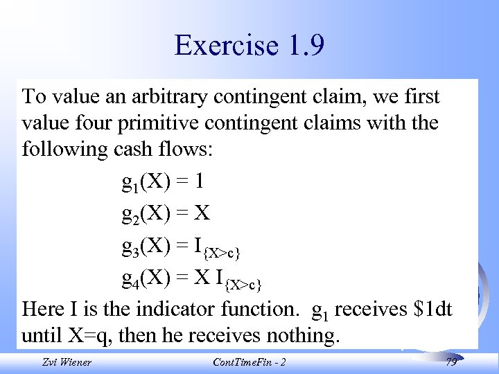Exercise 1. 9 To value an arbitrary contingent claim, we first value four primitive contingent claims with the following cash flows: g 1(X) = 1 g 2(X) = X g 3(X) = I{X>c} g 4(X) = X I{X>c} Here I is the indicator function. g 1 receives $1 dt until X=q, then he receives nothing. Zvi Wiener Cont. Time. Fin - 2 79

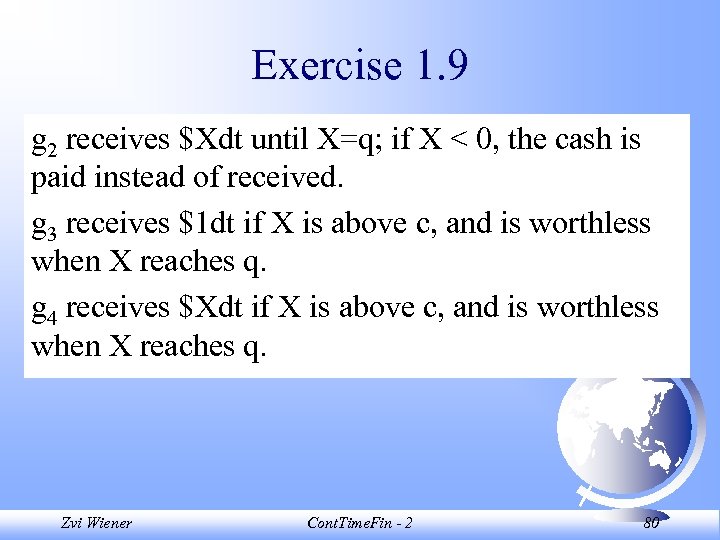Exercise 1. 9 g 2 receives $Xdt until X=q; if X < 0, the cash is paid instead of received. g 3 receives $1 dt if X is above c, and is worthless when X reaches q. g 4 receives $Xdt if X is above c, and is worthless when X reaches q. Zvi Wiener Cont. Time. Fin - 2 80

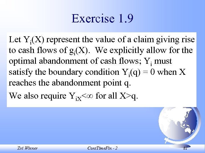Exercise 1. 9 Let Yi(X) represent the value of a claim giving rise to cash flows of gi(X). We explicitly allow for the optimal abandonment of cash flows; Yi must satisfy the boundary condition Yi(q) = 0 when X reaches the abandonment point q. We also require Yi. X< for all X>q. Zvi Wiener Cont. Time. Fin - 2 81

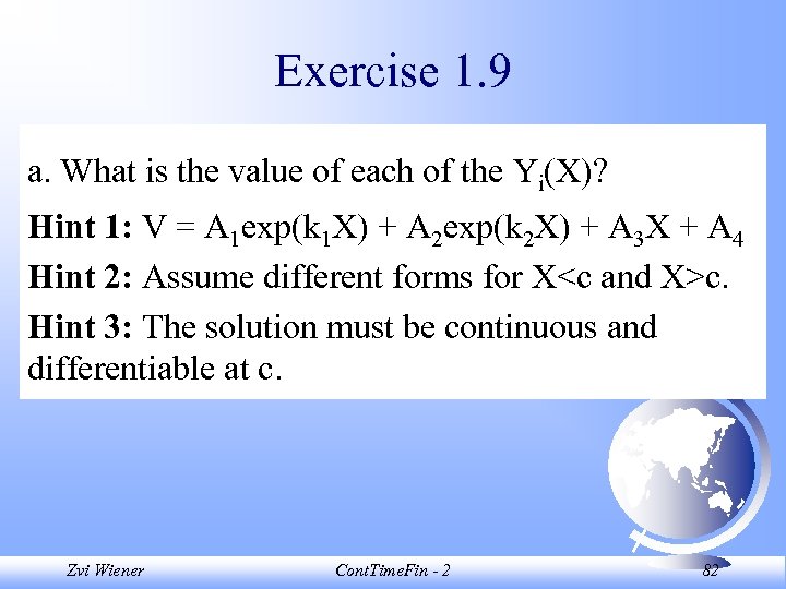Exercise 1. 9 a. What is the value of each of the Yi(X)? Hint 1: V = A 1 exp(k 1 X) + A 2 exp(k 2 X) + A 3 X + A 4 Hint 2: Assume different forms for Xc. Hint 3: The solution must be continuous and differentiable at c. Zvi Wiener Cont. Time. Fin - 2 82

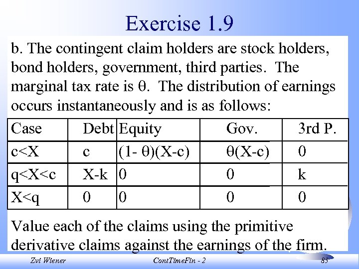Exercise 1. 9 b. The contingent claim holders are stock holders, bond holders, government, third parties. The marginal tax rate is . The distribution of earnings occurs instantaneously and is as follows: Case Debt Equity Gov. 3 rd P. c

Exercise 1. 9 c. Find the operating and capital structure policy (levels of q and c) that maximizes the sum of debt and equity values. Write down the first order conditions for an interior maximum only. Zvi Wiener Cont. Time. Fin - 2 84

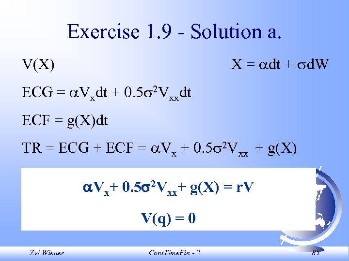Exercise 1. 9 - Solution a. X = dt + d. W V(X) ECG = Vxdt + 0. 5 2 Vxxdt ECF = g(X)dt TR = ECG + ECF = Vx + 0. 5 2 Vxx + g(X) Vx+ 0. 5 2 Vxx+ g(X) = r. V V(q) = 0 Zvi Wiener Cont. Time. Fin - 2 85

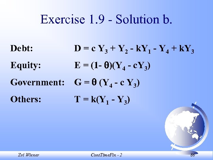Exercise 1. 9 - Solution b. Debt: D = c Y 3 + Y 2 - k. Y 1 - Y 4 + k. Y 3 Equity: E = (1 - )(Y 4 - c. Y 3) Government: G = (Y 4 - c Y 3) Others: T = k(Y 1 - Y 3) Zvi Wiener Cont. Time. Fin - 2 86