Final Review Econ 240 A 1 Outline

Final Review Econ 240 A 1

Outline n n n n The Big Picture Processes to remember ( and habits to form) for your quantitative career (FYQC) Concepts to remember FYQC Discrete Distributions Continuous distributions Central Limit Theorem Regression 2

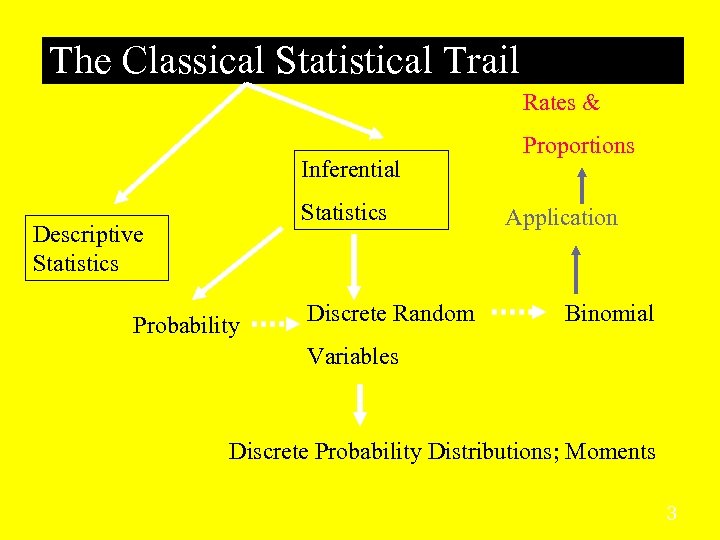The Classical Statistical Trail Rates & Inferential Statistics Descriptive Statistics Probability Discrete Random Proportions Application Binomial Variables Discrete Probability Distributions; Moments 3

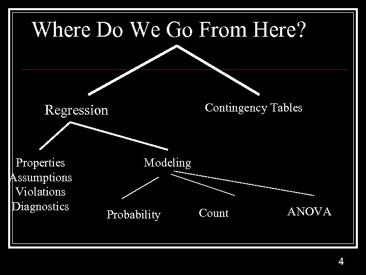Where Do We Go From Here? Contingency Tables Regression Properties Assumptions Violations Diagnostics Modeling Probability Count ANOVA 4

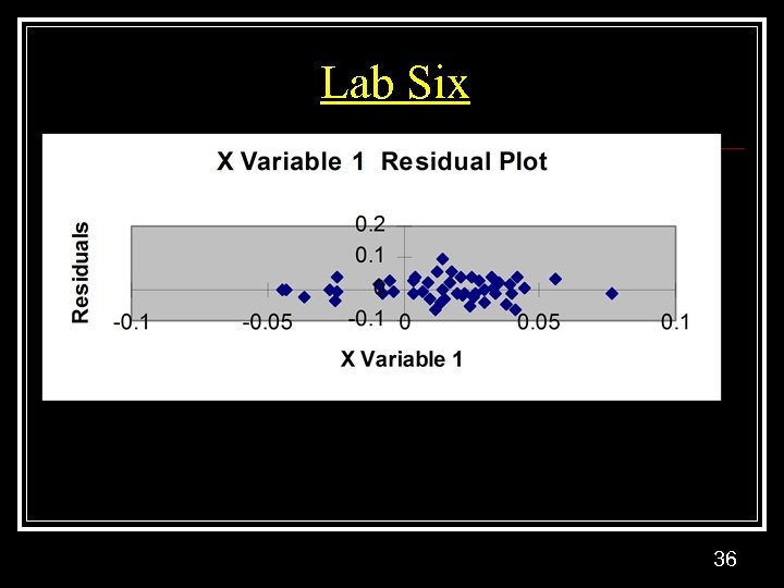
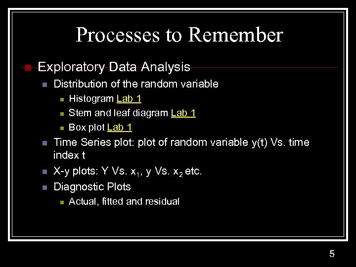Processes to Remember n Exploratory Data Analysis n Distribution of the random variable n n n Histogram Lab 1 Stem and leaf diagram Lab 1 Box plot Lab 1 Time Series plot: plot of random variable y(t) Vs. time index t X-y plots: Y Vs. x 1, y Vs. x 2 etc. Diagnostic Plots n Actual, fitted and residual 5

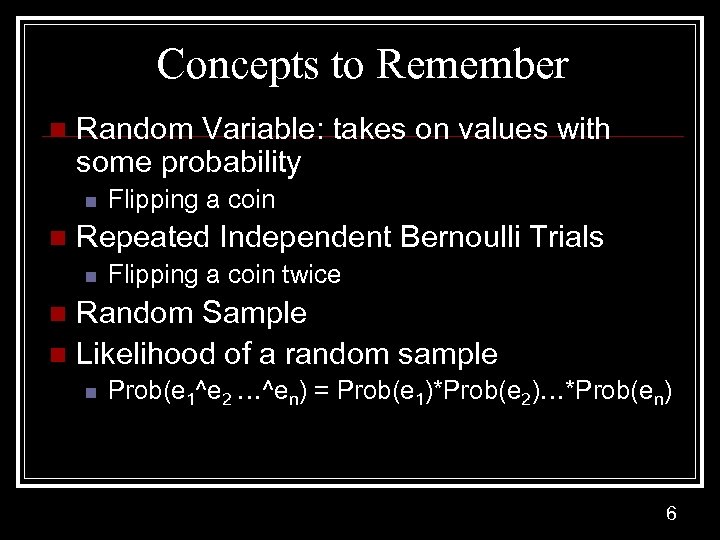Concepts to Remember n Random Variable: takes on values with some probability n n Flipping a coin Repeated Independent Bernoulli Trials n Flipping a coin twice Random Sample n Likelihood of a random sample n n Prob(e 1^e 2 …^en) = Prob(e 1)*Prob(e 2)…*Prob(en) 6

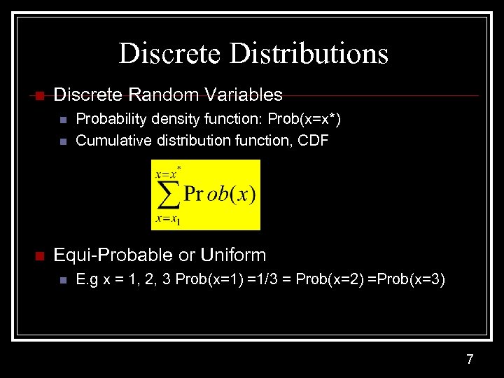Discrete Distributions n Discrete Random Variables n n n Probability density function: Prob(x=x*) Cumulative distribution function, CDF Equi-Probable or Uniform n E. g x = 1, 2, 3 Prob(x=1) =1/3 = Prob(x=2) =Prob(x=3) 7

Discrete Distributions n Binomial: Prob(k) = [n!/k!*(n-k)!]* pk (1 -p)n-k n n E(k) = n*p, Var(k) = n*p*(1 -p) Simulated sample binomial random variable Lab 2 Rates and proportions Poisson 8

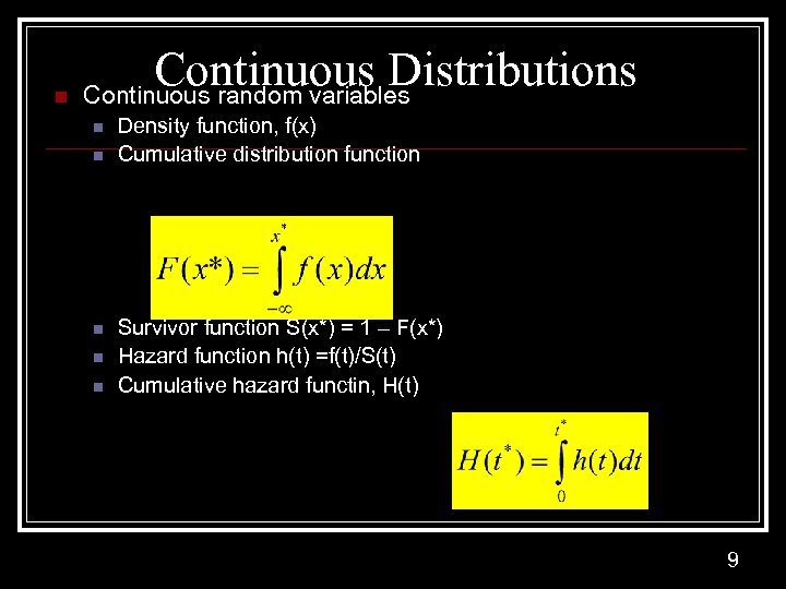n Continuous Distributions Continuous random variables n n n Density function, f(x) Cumulative distribution function Survivor function S(x*) = 1 – F(x*) Hazard function h(t) =f(t)/S(t) Cumulative hazard functin, H(t) 9

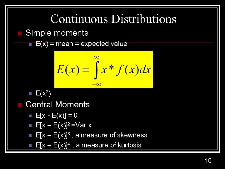Continuous Distributions n Simple moments n n n E(x) = mean = expected value E(x 2) Central Moments n n E[x - E(x)] = 0 E[x – E(x)]2 =Var x E[x – E(x)]3 , a measure of skewness E[x – E(x)]4 , a measure of kurtosis 10

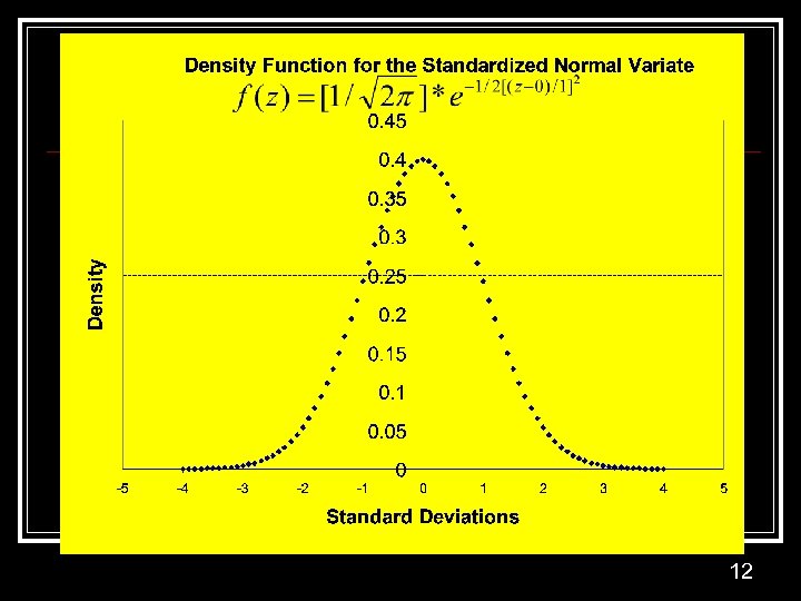
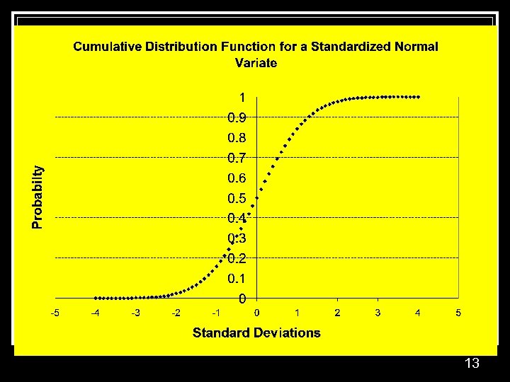
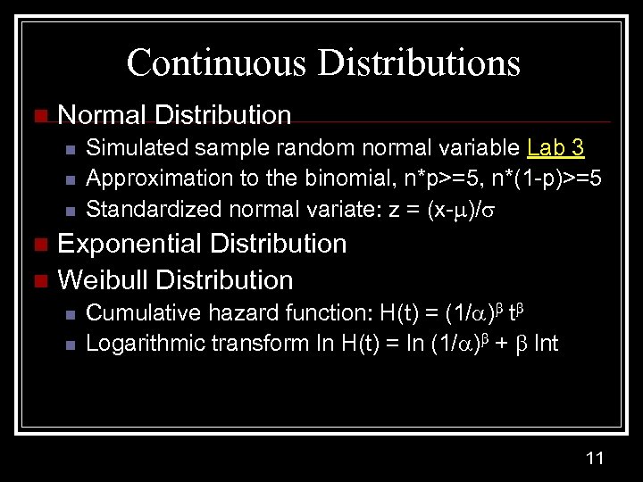Continuous Distributions n Normal Distribution n Simulated sample random normal variable Lab 3 Approximation to the binomial, n*p>=5, n*(1 -p)>=5 Standardized normal variate: z = (x- )/ Exponential Distribution n Weibull Distribution n Cumulative hazard function: H(t) = (1/ ) t Logarithmic transform ln H(t) = ln (1/ ) + lnt 11

12

13

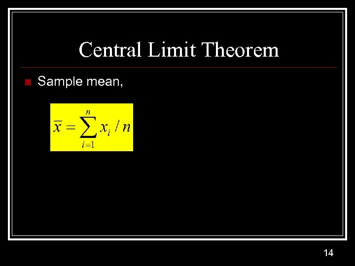Central Limit Theorem n Sample mean, 14

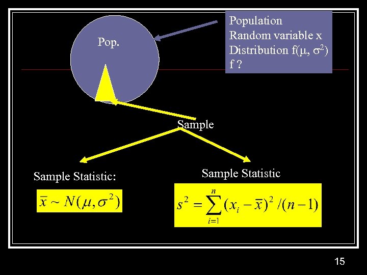Population Random variable x Distribution f( , 2) f? Pop. Sample Statistic: Sample Statistic 15

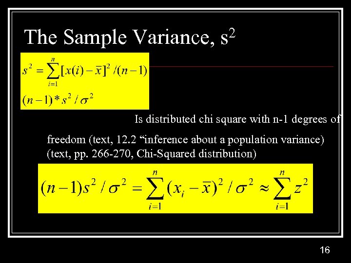The Sample Variance, s 2 Is distributed chi square with n-1 degrees of freedom (text, 12. 2 “inference about a population variance) (text, pp. 266 -270, Chi-Squared distribution) 16

Regression Models n Statistical distributions and tests n n Student’s t F Chi Square Assumptions n Pathologies n 17

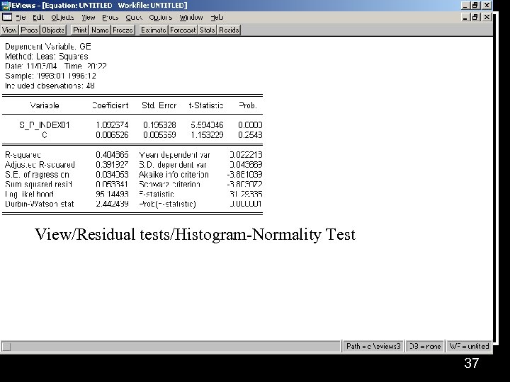
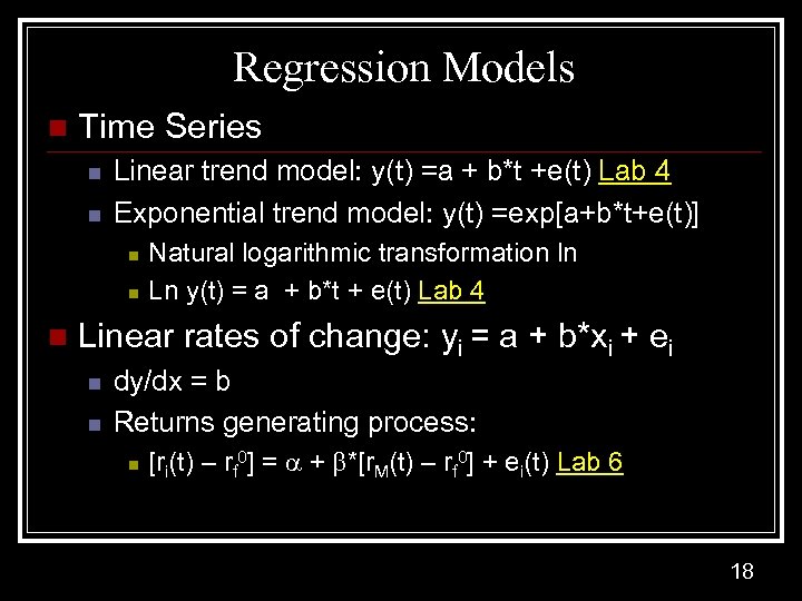Regression Models n Time Series n n Linear trend model: y(t) =a + b*t +e(t) Lab 4 Exponential trend model: y(t) =exp[a+b*t+e(t)] n n n Natural logarithmic transformation ln Ln y(t) = a + b*t + e(t) Lab 4 Linear rates of change: yi = a + b*xi + ei n n dy/dx = b Returns generating process: n [ri(t) – rf 0] = + *[r. M(t) – rf 0] + ei(t) Lab 6 18

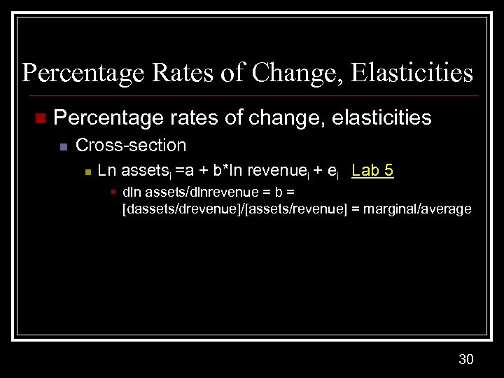
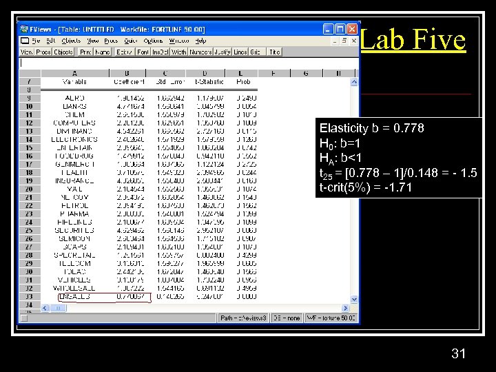
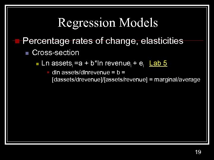Regression Models n Percentage rates of change, elasticities n Cross-section n Ln assetsi =a + b*ln revenuei + ei Lab 5 § dln assets/dlnrevenue = b = [dassets/drevenue]/[assets/revenue] = marginal/average 19

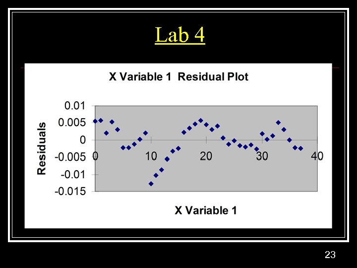
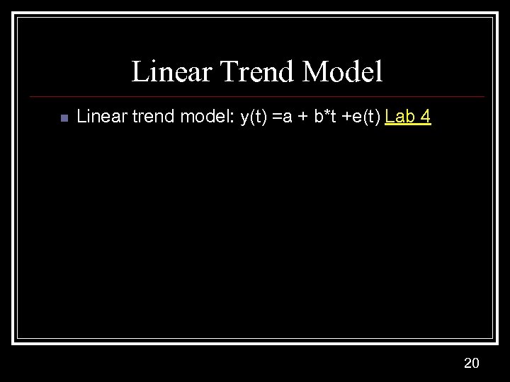Linear Trend Model n Linear trend model: y(t) =a + b*t +e(t) Lab 4 20

Lab 4 21

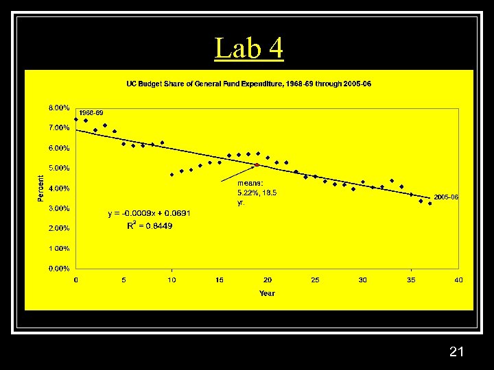
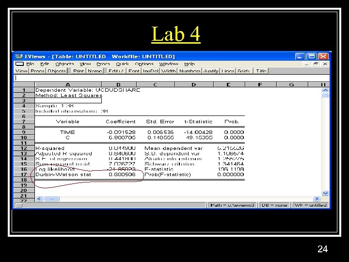
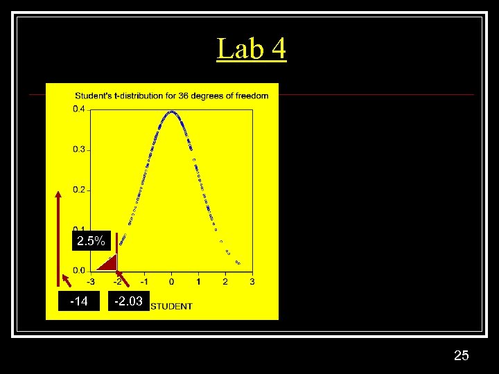
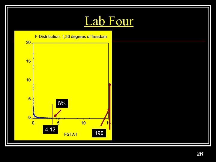
Lab Four F-test: F 1, 36 = [R 2/1]/{[1 -R 2]/36} = 196 = Explained Mean Square/Unexplained mean square t-test: H 0: b=0 HA: b≠ 0 t =[ -0. 000915 – 0]/0. 0000653 = -14 22

Lab 4 23

Lab 4 24

Lab 4 2. 5% -14 -2. 03 25

Lab Four 5% 4. 12 196 26

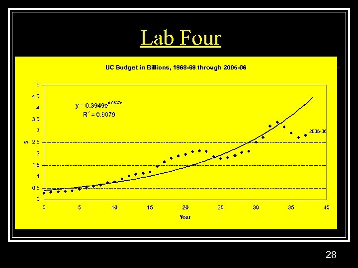
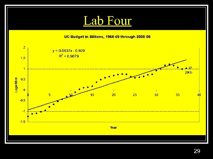
Exponential Trend Model n Exponential trend model: y(t) =exp[a+b*t+e(t)] n n Natural logarithmic transformation ln Ln y(t) = a + b*t + e(t) Lab 4 27

Lab Four 28

Lab Four 29

Percentage Rates of Change, Elasticities n Percentage rates of change, elasticities n Cross-section n Ln assetsi =a + b*ln revenuei + ei Lab 5 § dln assets/dlnrevenue = b = [dassets/drevenue]/[assets/revenue] = marginal/average 30

Lab Five Elasticity b = 0. 778 H 0: b=1 HA: b<1 t 25 = [0. 778 – 1]/0. 148 = - 1. 5 t-crit(5%) = -1. 71 31

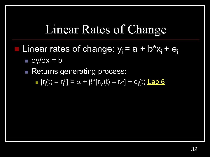Linear Rates of Change n Linear rates of change: yi = a + b*xi + ei n n dy/dx = b Returns generating process: n [ri(t) – rf 0] = + *[r. M(t) – rf 0] + ei(t) Lab 6 32

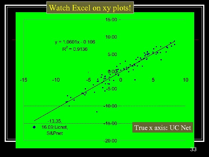Watch Excel on xy plots! True x axis: UC Net 33

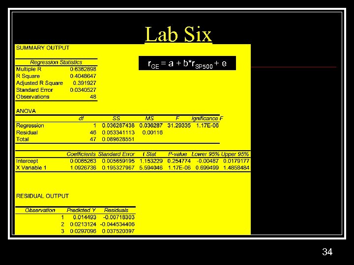Lab Six r. GE = a + b*r. SP 500 + e 34

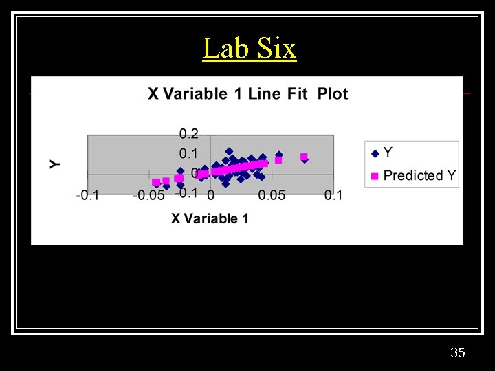Lab Six 35

Lab Six 36

View/Residual tests/Histogram-Normality Test 37

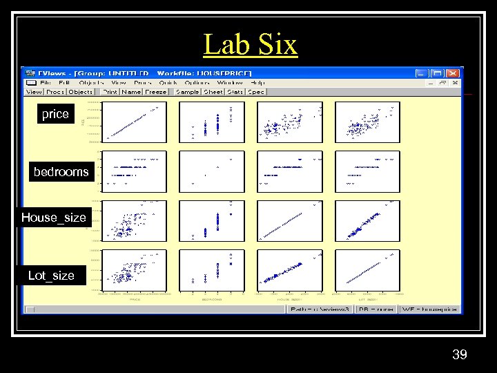
Linear Multivariate Regression n House Price, # of bedrooms, house size, lot size n Pi = a + b*bedroomsi + c*house_sizei + d*lot_sizei + ei 38

Lab Six price bedrooms House_size Lot_size 39

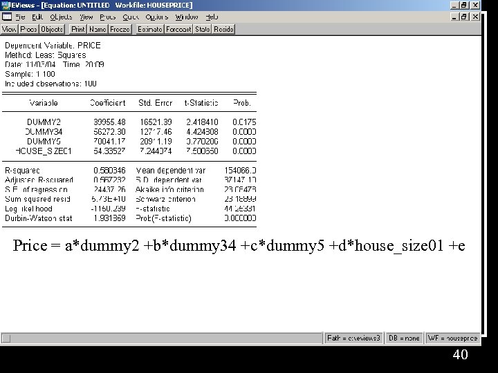Price = a*dummy 2 +b*dummy 34 +c*dummy 5 +d*house_size 01 +e 40

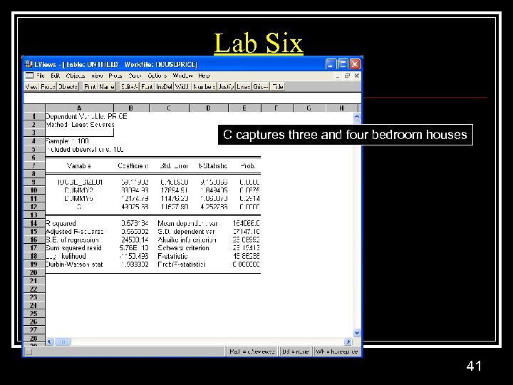Lab Six C captures three and four bedroom houses 41

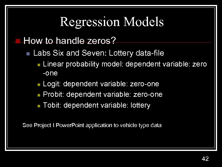Regression Models n How to handle zeros? n Labs Six and Seven: Lottery data-file n n Linear probability model: dependent variable: zero -one Logit: dependent variable: zero-one Probit: dependent variable: zero-one Tobit: dependent variable: lottery See Project I Power. Point application to vehicle type data 42

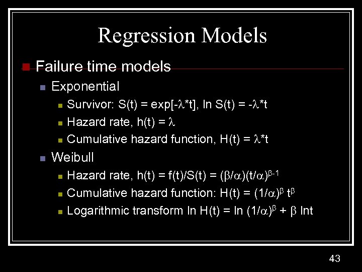Regression Models n Failure time models n Exponential n n Survivor: S(t) = exp[- *t], ln S(t) = - *t Hazard rate, h(t) = Cumulative hazard function, H(t) = *t Weibull n n n Hazard rate, h(t) = f(t)/S(t) = ( / )(t/ ) -1 Cumulative hazard function: H(t) = (1/ ) t Logarithmic transform ln H(t) = ln (1/ ) + lnt 43