FIN 30220 Macroeconomic Analysis Using Economic Data

FIN 30220: Macroeconomic Analysis Using Economic Data

“There are three kinds of lies; Lies, Damn Lies, and Statistics” - Mark Twain

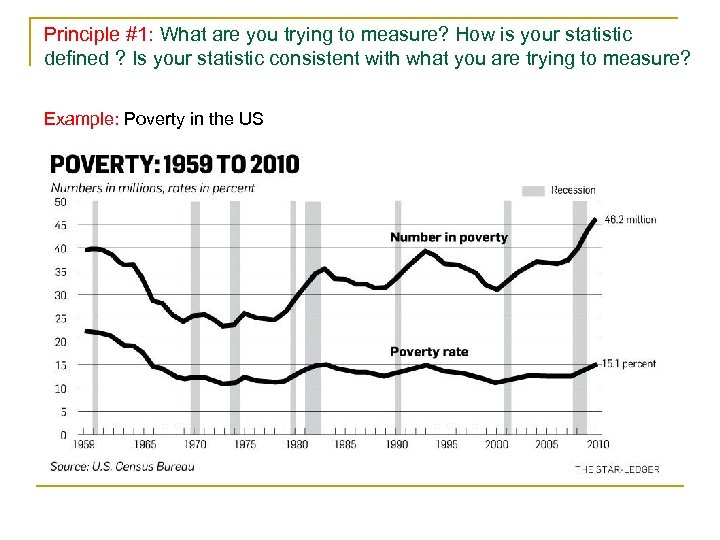Principle #1: What are you trying to measure? How is your statistic defined ? Is your statistic consistent with what you are trying to measure? Example: Poverty in the US

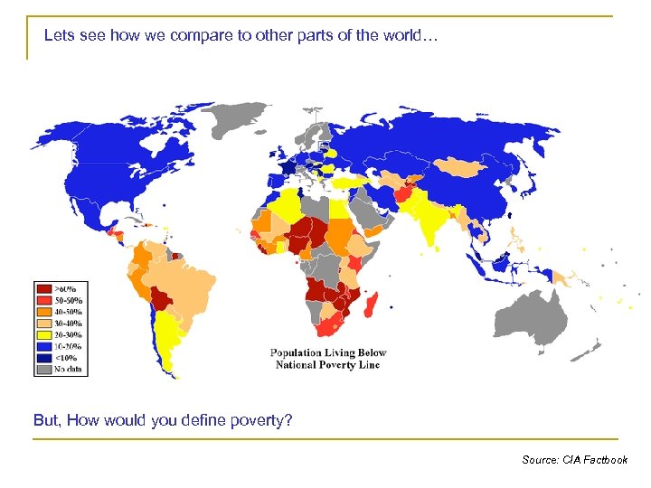Lets see how we compare to other parts of the world… But, How would you define poverty? Source: CIA Factbook

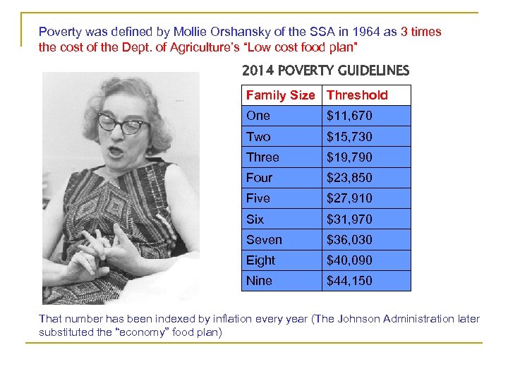Poverty was defined by Mollie Orshansky of the SSA in 1964 as 3 times the cost of the Dept. of Agriculture’s “Low cost food plan” 2014 POVERTY GUIDELINES Family Size Threshold One $11, 670 Two $15, 730 Three $19, 790 Four $23, 850 Five $27, 910 Six $31, 970 Seven $36, 030 Eight $40, 090 Nine $44, 150 That number has been indexed by inflation every year (The Johnson Administration later substituted the “economy” food plan)

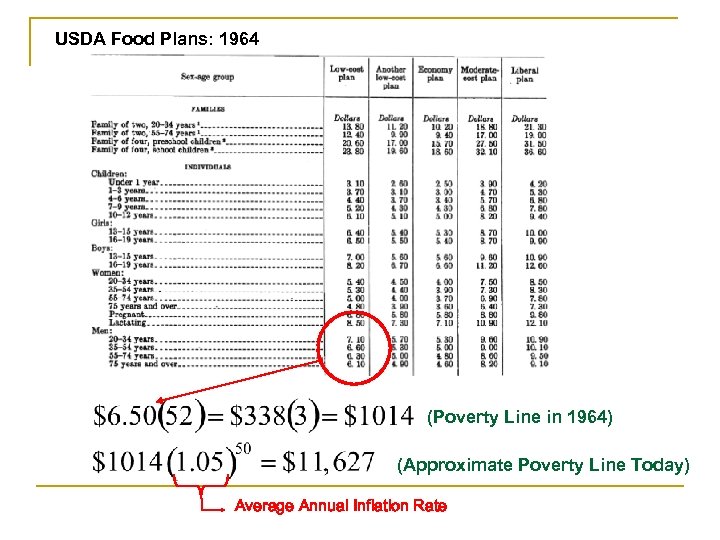USDA Food Plans: 1964 (Poverty Line in 1964) (Approximate Poverty Line Today) Average Annual Inflation Rate

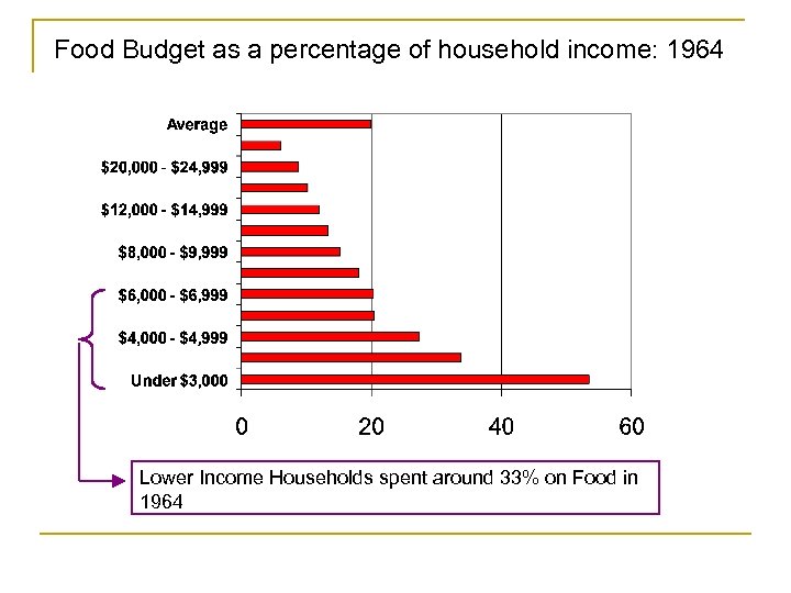Food Budget as a percentage of household income: 1964 Lower Income Households spent around 33% on Food in 1964

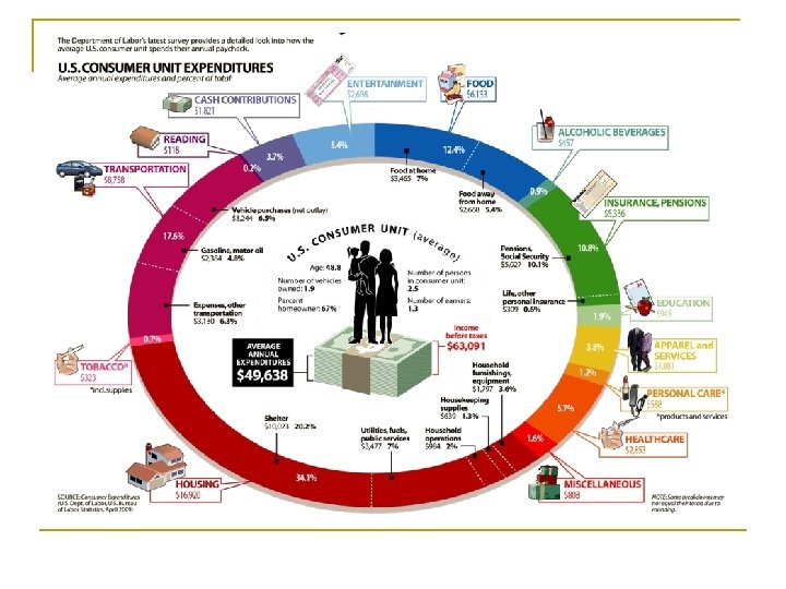
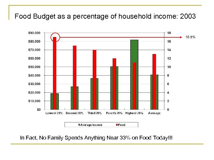Food Budget as a percentage of household income: 2003 16. 5% In Fact, No Family Spends Anything Near 33% on Food Today!!!

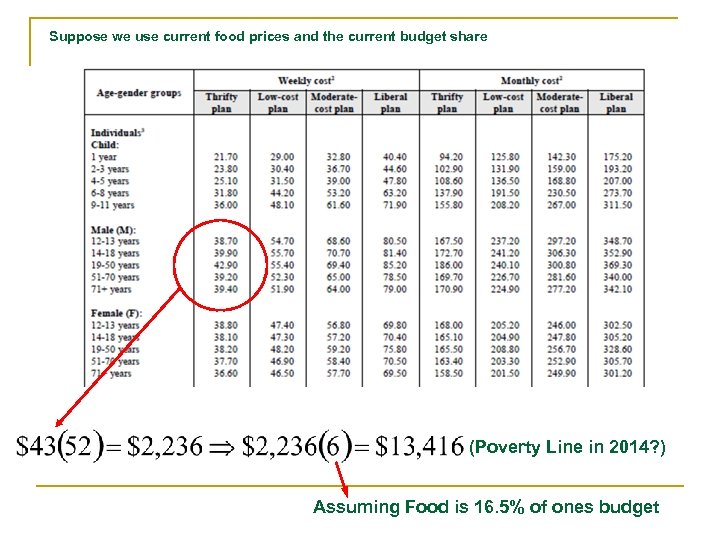Suppose we use current food prices and the current budget share (Poverty Line in 2014? ) Assuming Food is 16. 5% of ones budget

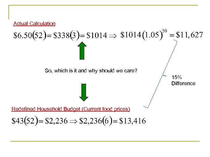Actual Calculation So, which is it and why should we care? 15% Difference Redefined Household Budget (Current food prices)

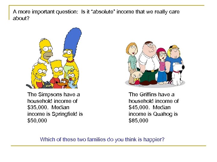A more important question: Is it “absolute” income that we really care about? The Simpsons have a household income of $35, 000. Median income is Springfield is $50, 000 The Griffins have a household income of $45, 000. Median income is Quahog is $85, 000 Which of these two families do you think is happier?

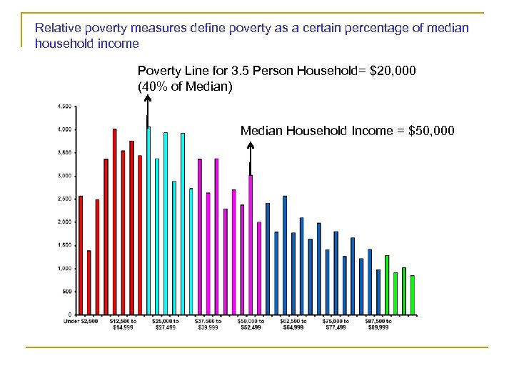Relative poverty measures define poverty as a certain percentage of median household income Poverty Line for 3. 5 Person Household= $20, 000 (40% of Median) Median Household Income = $50, 000

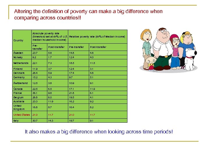Altering the definition of poverty can make a big difference when comparing across countries!! Absolute poverty rate (threshold set at 40% of U. S. Relative poverty rate (40% of Median Income) median household income) Country Pretransfer Post-transfer Pre-transfer Post-transfer Sweden 23. 7 5. 8 14. 8 Norway 9. 2 1. 7 12. 4 4. 0 Netherlands 22. 1 7. 3 18. 5 11. 5 Finland 11. 9 3. 7 12. 4 3. 1 Denmark 26. 4 5. 9 17. 4 4. 8 Germany 15. 2 4. 3 9. 7 5. 1 Switzerland 12. 5 3. 8 10. 9 9. 1 Canada 22. 5 6. 5 17. 1 11. 9 France 36. 1 9. 8 21. 8 6. 1 Belgium 26. 8 6. 0 19. 5 4. 1 Australia 23. 3 11. 9 16. 2 9. 2 United Kingdom 16. 8 8. 7 16. 4 8. 2 United States 21. 0 11. 7 Italy 14. 3 19. 7 9. 1 30. 7 It also makes a big difference when looking across time periods!

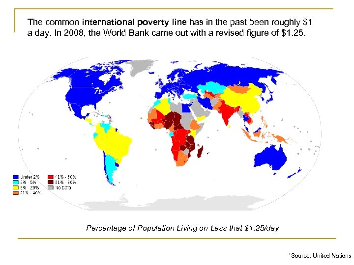The common international poverty line has in the past been roughly $1 a day. In 2008, the World Bank came out with a revised figure of $1. 25. Percentage of Population Living on Less that $1. 25/day *Source: United Nations

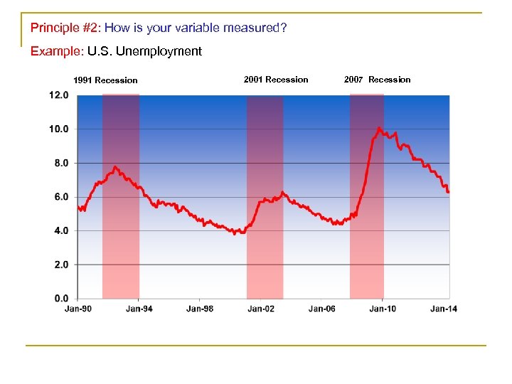Principle #2: How is your variable measured? Example: U. S. Unemployment 1991 Recession 2007 Recession

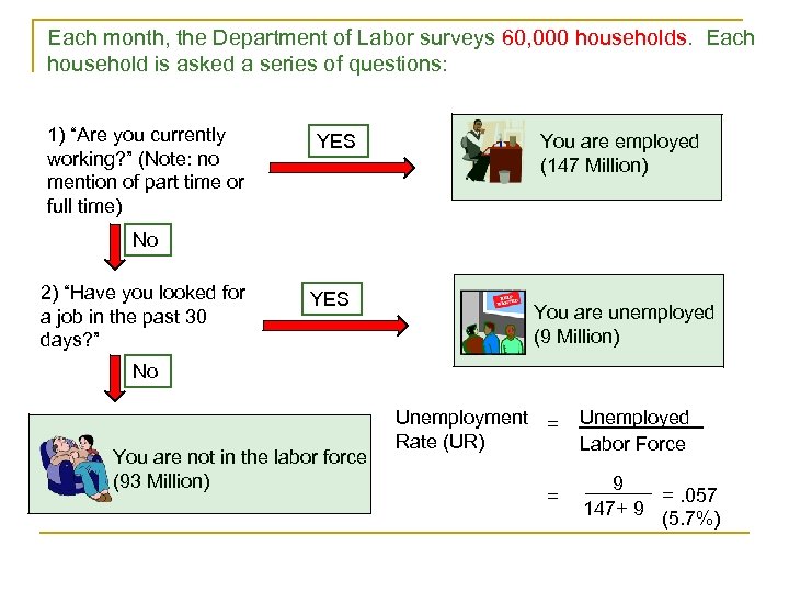Each month, the Department of Labor surveys 60, 000 households. Each household is asked a series of questions: 1) “Are you currently working? ” (Note: no mention of part time or full time) YES You are employed (147 Million) No 2) “Have you looked for a job in the past 30 days? ” YES You are unemployed (9 Million) No You are not in the labor force (93 Million) Unemployment = Rate (UR) = Unemployed Labor Force 9 =. 057 147+ 9 (5. 7%)

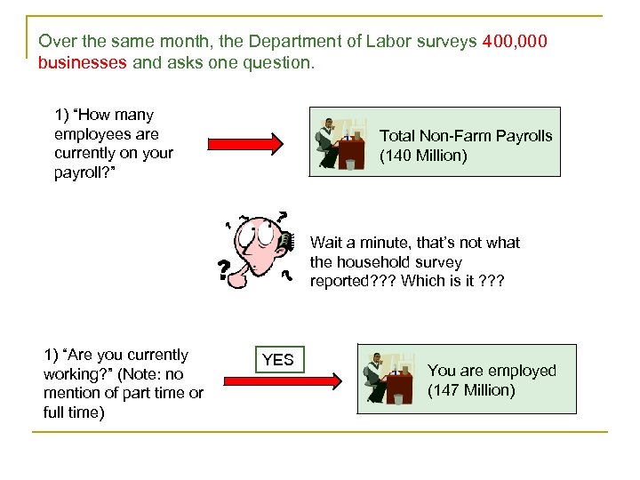Over the same month, the Department of Labor surveys 400, 000 businesses and asks one question. 1) “How many employees are currently on your payroll? ” Total Non-Farm Payrolls (140 Million) Wait a minute, that’s not what the household survey reported? ? ? Which is it ? ? ? 1) “Are you currently working? ” (Note: no mention of part time or full time) YES You are employed (147 Million)

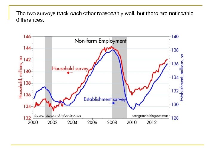The two surveys track each other reasonably well, but there are noticeable differences.

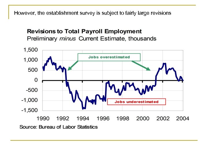However, the establishment survey is subject to fairly large revisions

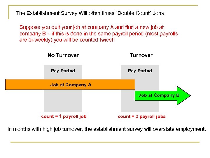The Establishment Survey Will often times “Double Count” Jobs Suppose you quit your job at company A and find a new job at company B – if this is done in the same payroll period (most payrolls are bi-weekly) you will be counted twice!! No Turnover Pay Period Job at Company A Job at Company B count = 1 payroll job count = 2 payroll jobs In months with high job turnover, the establishment survey will overstate employment.

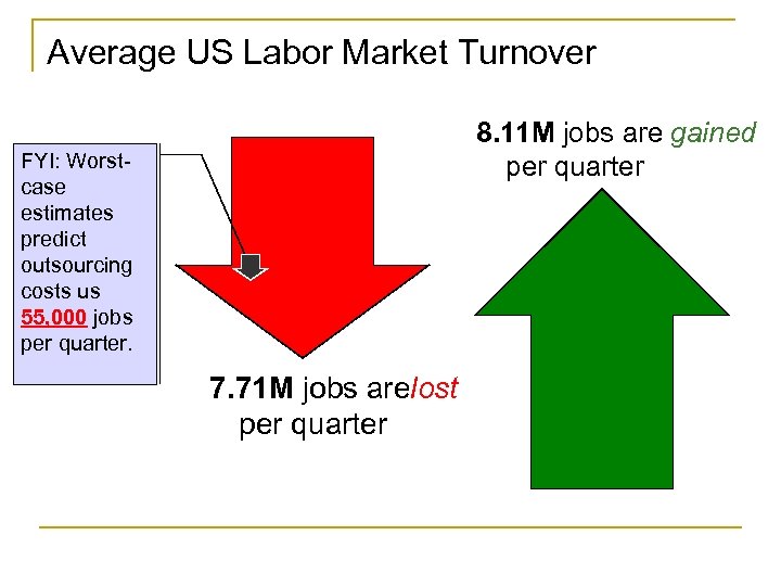Average US Labor Market Turnover 8. 11 M jobs are gained per quarter FYI: Worstcase estimates predict outsourcing costs us 55, 000 jobs per quarter. 7. 71 M jobs arelost per quarter

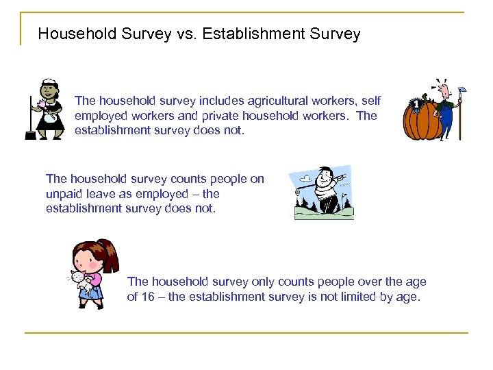Household Survey vs. Establishment Survey The household survey includes agricultural workers, self employed workers and private household workers. The establishment survey does not. The household survey counts people on unpaid leave as employed – the establishment survey does not. The household survey only counts people over the age of 16 – the establishment survey is not limited by age.

Main problems with measuring the unemployment rate Ø Ø The unemployment rate doesn’t count underemployment (those that would like to work full time, but only work part time) The “discouraged worker effect”: Those that have given up trying to find a job are counted as not in the labor force rather than unemployed Selection bias: those that are unemployed are more likely to answer the survey. Moral hazard: due to unemployment insurance, it is difficult to tell how hard individuals are trying to find work

Principle #3: Is your variable in terms of current prices or fixed prices (Real vs. Nominal) Example: The Top 10 All Time Grossing Films (in Millions – US) 1) Avatar (2009): $760 2) Titanic(1997): $658 3) Marvel’s the Avengers (2012): $588 4) The Dark Knight (2008): $533 5) Star Wars I: The Phantom Menace (1999) $474 6) Star Wars IV: A New Hope (1977): $460 7) The Dark Knight Rises (2012) $449 8) Shrek 2 (2011): $441 9) E. T. The Extra-Terrestrial (1982): $435 10) The Hunger Games: Catching Fire (2013): $424

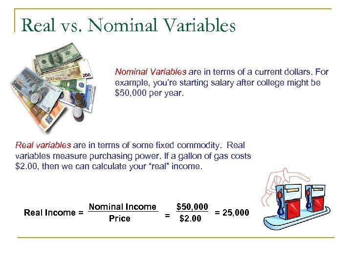Real vs. Nominal Variables are in terms of a current dollars. For example, you’re starting salary after college might be $50, 000 per year. Real variables are in terms of some fixed commodity. Real variables measure purchasing power. If a gallon of gas costs $2. 00, then we can calculate your “real” income. Real Income = Nominal Income $50, 000 = $2. 00 = 25, 000 Price

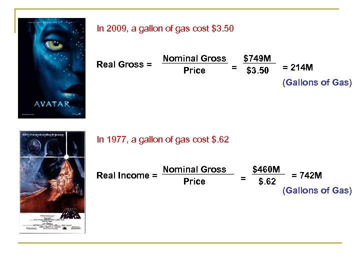In 2009, a gallon of gas cost $3. 50 Real Gross = Nominal Gross $749 M = $3. 50 Price = 214 M (Gallons of Gas) In 1977, a gallon of gas cost $. 62 Real Income = Nominal Gross Price $460 M = $. 62 = 742 M (Gallons of Gas)

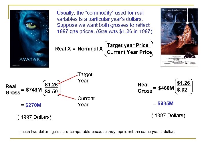Usually, the “commodity” used for real variables is a particular year’s dollars. Suppose we want both grosses to reflect 1997 gas prices. (Gas was $1. 26 in 1997) Real X = Nominal X $1. 26 Real = $749 M $3. 50 Gross = $270 M ( 1997 Dollars) Target Year Current Year Target year Price Current Year Price $1. 26 Real = $460 M $. 62 Gross = $935 M ( 1997 Dollars) These two dollar figures are comparable because they represent the same year’s dollars!

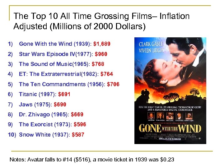The Top 10 All Time Grossing Films– Inflation Adjusted (Millions of 2000 Dollars) 1) Gone With the Wind (1939): $1, 689 2) Star Wars Episode IV(1977): $960 3) The Sound of Music(1965): $768 4) ET: The Extraterrestrial(1982): $764 5) The Ten Commandments (1956): $706 6) Titanic (1997): $691 7) Jaws (1975): $690 8) Dr. Zhivago (1965): $669 9) The Exorcist (1973): $596 10) Snow White (1937): $587 Notes: Avatar falls to #14 ($516), a movie ticket in 1939 was $0. 23

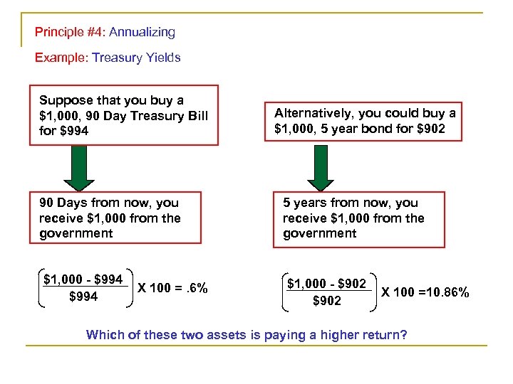Principle #4: Annualizing Example: Treasury Yields Suppose that you buy a $1, 000, 90 Day Treasury Bill for $994 90 Days from now, you receive $1, 000 from the government $1, 000 - $994 X 100 =. 6% Alternatively, you could buy a $1, 000, 5 year bond for $902 5 years from now, you receive $1, 000 from the government $1, 000 - $902 X 100 =10. 86% Which of these two assets is paying a higher return?

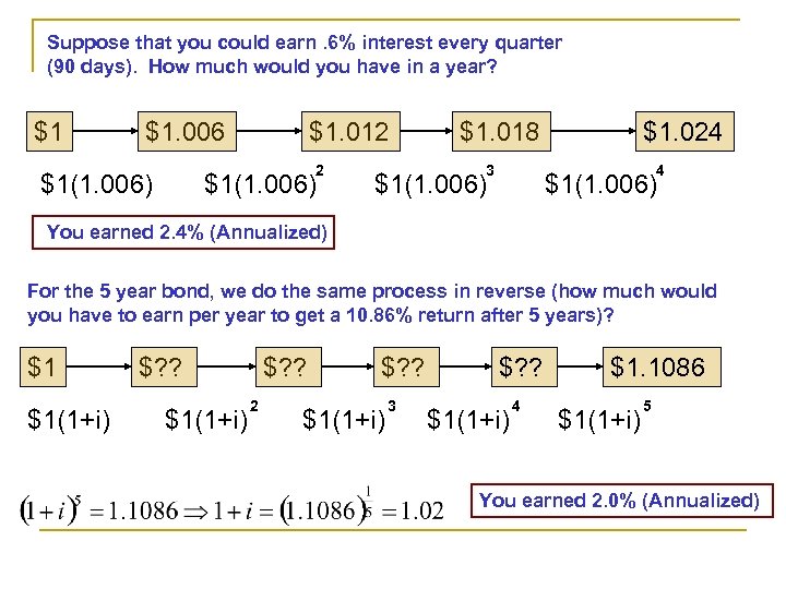Suppose that you could earn. 6% interest every quarter (90 days). How much would you have in a year? $1 $1. 006 $1. 012 2 $1(1. 006) $1. 018 3 $1. 024 4 $1(1. 006) You earned 2. 4% (Annualized) For the 5 year bond, we do the same process in reverse (how much would you have to earn per year to get a 10. 86% return after 5 years)? $1 $1(1+i) $? ? 2 $? ? $1(1+i) 3 $? ? $1(1+i) 4 $1. 1086 $1(1+i) 5 You earned 2. 0% (Annualized)

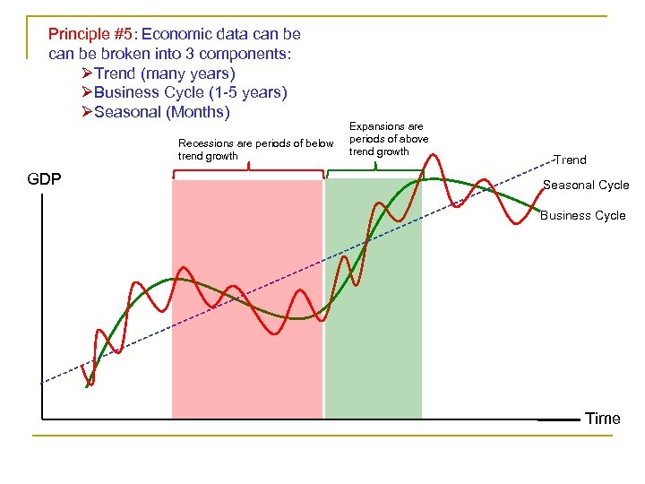Principle #5: Economic data can be broken into 3 components: ØTrend (many years) ØBusiness Cycle (1 -5 years) ØSeasonal (Months) Expansions are Recessions are periods of below periods of above trend growth GDP Trend Seasonal Cycle Business Cycle Time

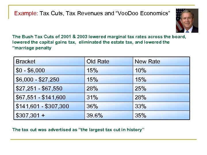Example: Tax Cuts, Tax Revenues and “Voo. Doo Economics” The Bush Tax Cuts of 2001 & 2003 lowered marginal tax rates across the board, lowered the capital gains tax, eliminated the estate tax, and lowered the “marriage penalty Bracket Old Rate New Rate $0 - $6, 000 15% 10% $6, 000 - $27, 250 15% $27, 251 - $67, 550 28% 25% $67, 551 - $141, 600 31% 28% $141, 601 - $307, 300 36% 33% $307, 301 + 39. 6% 35% The tax cut was advertised as “the largest tax cut in history”

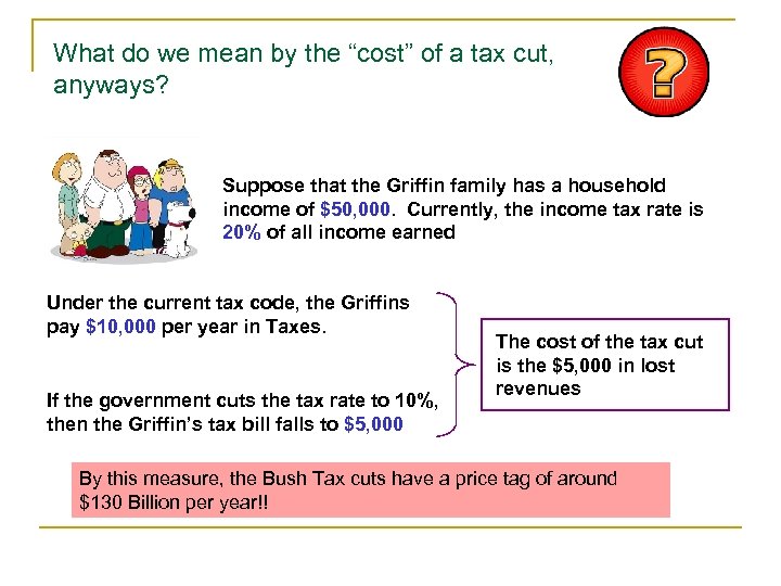What do we mean by the “cost” of a tax cut, anyways? Suppose that the Griffin family has a household income of $50, 000. Currently, the income tax rate is 20% of all income earned Under the current tax code, the Griffins pay $10, 000 per year in Taxes. If the government cuts the tax rate to 10%, then the Griffin’s tax bill falls to $5, 000 The cost of the tax cut is the $5, 000 in lost revenues By this measure, the Bush Tax cuts have a price tag of around $130 Billion per year!!

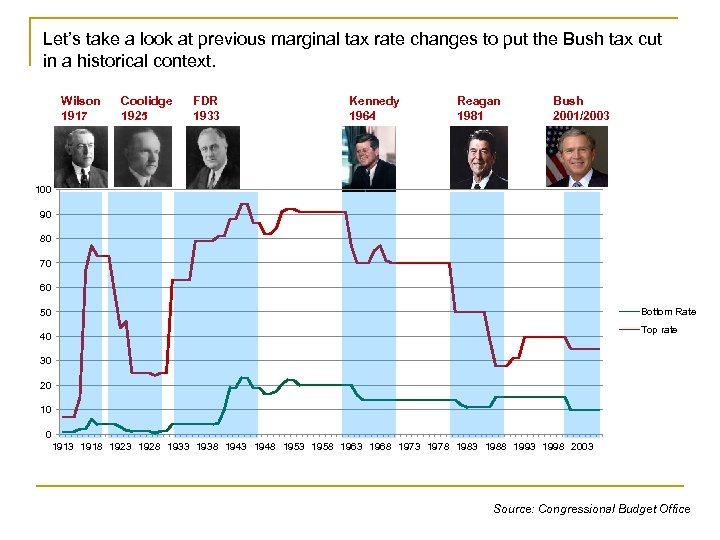Let’s take a look at previous marginal tax rate changes to put the Bush tax cut in a historical context. Wilson 1917 Coolidge 1925 FDR 1933 Kennedy 1964 Reagan 1981 Bush 2001/2003 100 90 80 70 60 Bottom Rate 50 Top rate 40 30 20 10 0 1913 1918 1923 1928 1933 1938 1943 1948 1953 1958 1963 1968 1973 1978 1983 1988 1993 1998 2003 Source: Congressional Budget Office

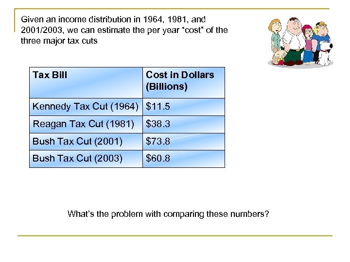Given an income distribution in 1964, 1981, and 2001/2003, we can estimate the per year “cost” of the three major tax cuts Tax Bill Cost in Dollars (Billions) Kennedy Tax Cut (1964) $11. 5 Reagan Tax Cut (1981) $38. 3 Bush Tax Cut (2001) $73. 8 Bush Tax Cut (2003) $60. 8 What’s the problem with comparing these numbers?

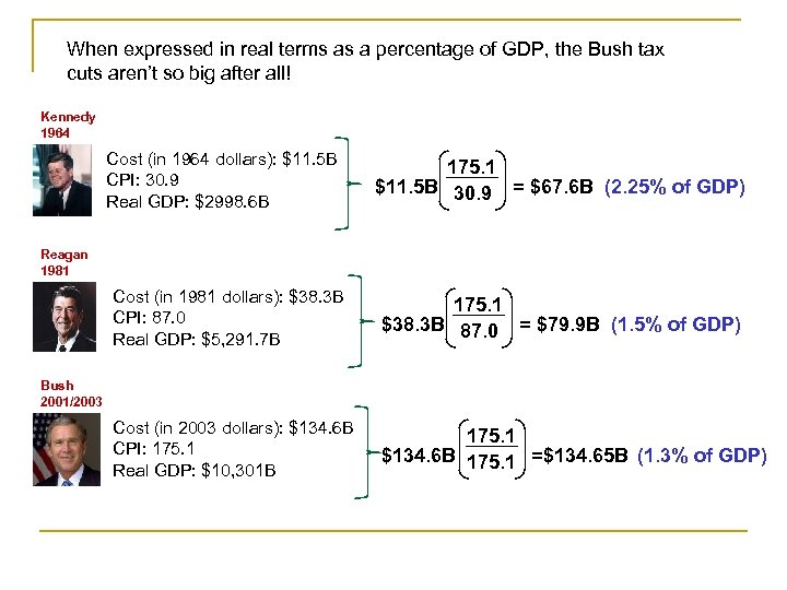When expressed in real terms as a percentage of GDP, the Bush tax cuts aren’t so big after all! Kennedy 1964 Cost (in 1964 dollars): $11. 5 B CPI: 30. 9 Real GDP: $2998. 6 B 175. 1 $11. 5 B 30. 9 = $67. 6 B (2. 25% of GDP) Reagan 1981 Cost (in 1981 dollars): $38. 3 B CPI: 87. 0 Real GDP: $5, 291. 7 B 175. 1 $38. 3 B 87. 0 = $79. 9 B (1. 5% of GDP) Cost (in 2003 dollars): $134. 6 B CPI: 175. 1 Real GDP: $10, 301 B 175. 1 $134. 6 B 175. 1 =$134. 65 B (1. 3% of GDP) Bush 2001/2003

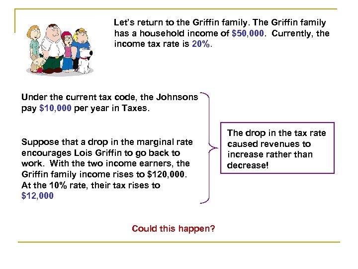Let’s return to the Griffin family. The Griffin family has a household income of $50, 000. Currently, the income tax rate is 20%. Under the current tax code, the Johnsons pay $10, 000 per year in Taxes. Suppose that a drop in the marginal rate encourages Lois Griffin to go back to work. With the two income earners, the Griffin family income rises to $120, 000. At the 10% rate, their tax rises to $12, 000 Could this happen? The drop in the tax rate caused revenues to increase rather than decrease!

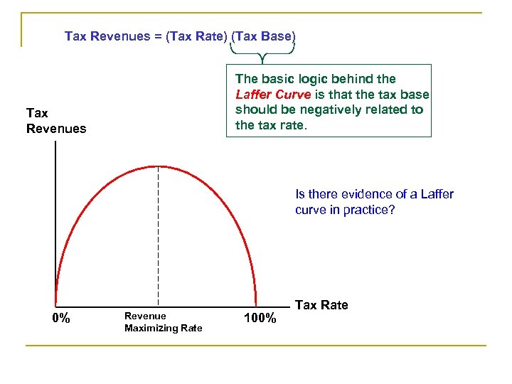Tax Revenues = (Tax Rate) (Tax Base) The basic logic behind the Laffer Curve is that the tax base should be negatively related to the tax rate. Tax Revenues Is there evidence of a Laffer curve in practice? 0% Revenue Maximizing Rate 100% Tax Rate

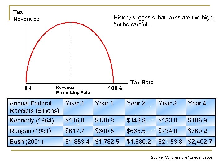Tax Revenues 0% History suggests that taxes are two high, but be careful… Revenue Maximizing Rate 100% Tax Rate Annual Federal Receipts (Billions) Year 0 Year 1 Year 2 Year 3 Year 4 Kennedy (1964) $116. 8 $130. 8 $148. 8 $153. 0 $186. 9 Reagan (1981) $617. 7 $600. 5 $666. 5 $734. 0 $769. 2 Bush (2001) $1, 853. 4 $1, 782. 5 $1, 880. 2 $2, 153. 8 $2, 402. 7 Source: Congressional Budget Office

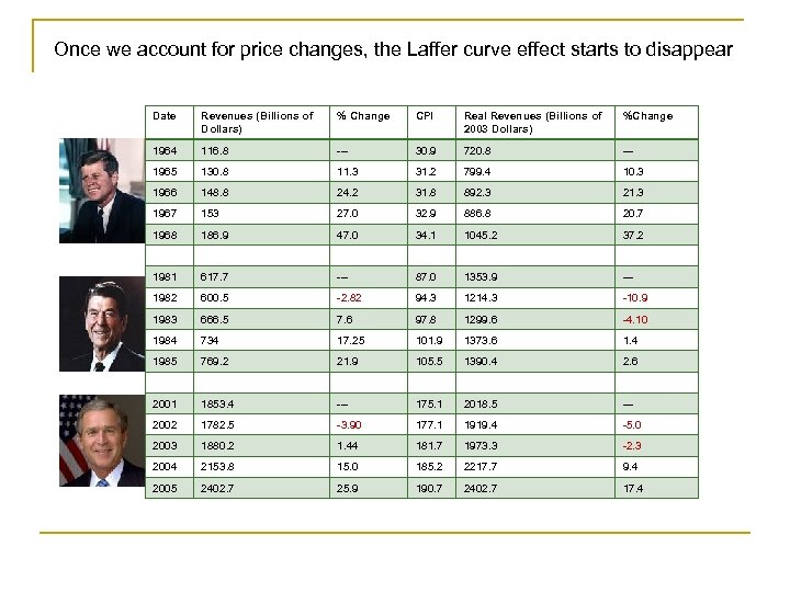Once we account for price changes, the Laffer curve effect starts to disappear Date Revenues (Billions of Dollars) % Change CPI Real Revenues (Billions of 2003 Dollars) %Change 1964 116. 8 --- 30. 9 720. 8 --- 1965 130. 8 11. 3 31. 2 799. 4 10. 3 1966 148. 8 24. 2 31. 8 892. 3 21. 3 1967 153 27. 0 32. 9 886. 8 20. 7 1968 186. 9 47. 0 34. 1 1045. 2 37. 2 1981 617. 7 --- 87. 0 1353. 9 --- 1982 600. 5 -2. 82 94. 3 1214. 3 -10. 9 1983 666. 5 7. 6 97. 8 1299. 6 -4. 10 1984 734 17. 25 101. 9 1373. 6 1. 4 1985 769. 2 21. 9 105. 5 1390. 4 2. 6 2001 1853. 4 --- 175. 1 2018. 5 --- 2002 1782. 5 -3. 90 177. 1 1919. 4 -5. 0 2003 1880. 2 1. 44 181. 7 1973. 3 -2. 3 2004 2153. 8 15. 0 185. 2 2217. 7 9. 4 2005 2402. 7 25. 9 190. 7 2402. 7 17. 4

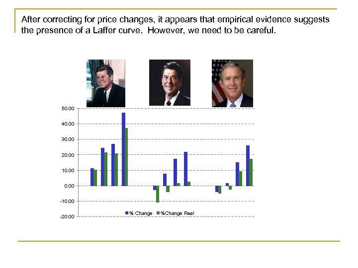After correcting for price changes, it appears that empirical evidence suggests the presence of a Laffer curve. However, we need to be careful. 50. 00 40. 00 30. 00 20. 00 10. 00 -10. 00 -20. 00 % Change %Change Real

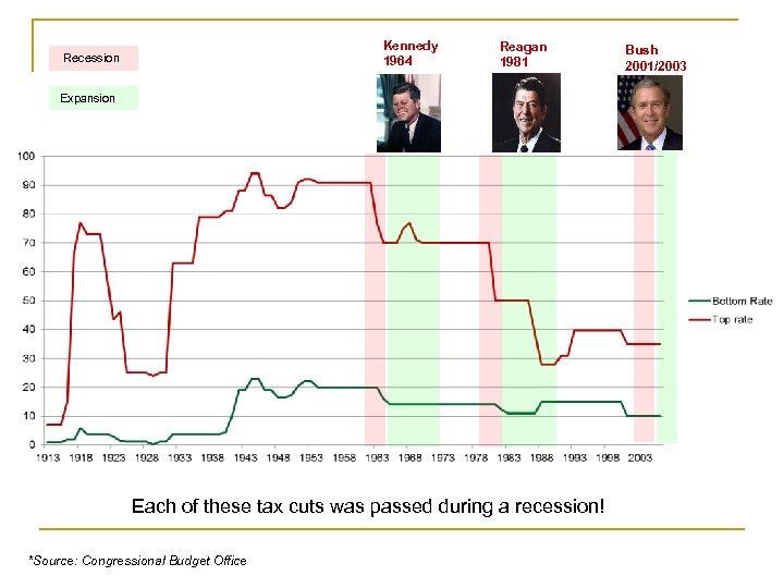Kennedy 1964 Recession Reagan 1981 Expansion Each of these tax cuts was passed during a recession! *Source: Congressional Budget Office Bush 2001/2003

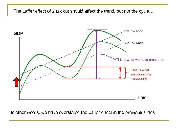The Laffer effect of a tax cut should affect the trend, but not the cycle… GDP New Tax Code Old Tax Code This is what we have measured This is what we should be measuring Time In other words, we have overstated the Laffer effect in the previous slides