Fast Algorithms for Time Series with applications to

Fast Algorithms for Time Series with applications to Finance, Physics, Music and other Suspects Dennis Shasha Joint work with Yunyue Zhu, Xiaojian Zhao, Zhihua Wang, and Alberto Lerner {shasha, yunyue, xiaojian, zhihua, lerner}@cs. nyu. edu Courant Institute, New York University

Goal of this work • Time series are important in so many applications – biology, medicine, finance, music, physics, … • A few fundamental operations occur all the time: burst detection, correlation, pattern matching. • Do them fast to make data exploration faster, real time, and more fun. 2

Sample Needs • Pairs Trading in Finance: find two stocks that track one another closely. When they go out of correlation, buy one and sell the other. • Match a person’s humming against a database of songs to help him/her buy a song. • Find bursts of activity even when you don’t know the window size over which to measure. • Query and manipulate ordered data. 3

Why Speed Is Important • Person on the street: “As processors speed up, algorithmic efficiency no longer matters” • True if problem sizes stay same. • They don’t. As processors speed up, sensors improve – e. g. satellites spewing out a terabyte a day, magnetic resonance imagers give higher resolution images, etc. • Desire for real time response to queries. 4

Surprise, surprise • More data, real-time response, increasing importance of correlation IMPLIES Efficient algorithms and data management more important than ever! 5

Corollary • Important area, lots of new problems. • Small advertisement: High Performance Discovery in Time Series (Springer 2004). At this conference. 6

Outline • Correlation across thousands of time series • Query by humming: correlation + shifting • Burst detection: when you don’t know window size • Aquery: a query language for time series. 7

Real-time Correlation Across Thousands (and scaling) of Time Series

Scalable Methods for Correlation • Compress streaming data into moving synopses. • Update the synopses in constant time. • Compare synopses in near linear time with respect to number of time series. • Use transforms + simple data structures. (Avoid curse of dimensionality. ) 9

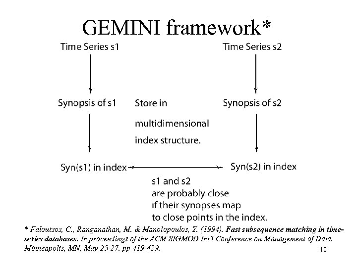GEMINI framework* * Faloutsos, C. , Ranganathan, M. & Manolopoulos, Y. (1994). Fast subsequence matching in timeseries databases. In proceedings of the ACM SIGMOD Int'l Conference on Management of Data. Minneapolis, MN, May 25 -27. pp 419 -429. 10

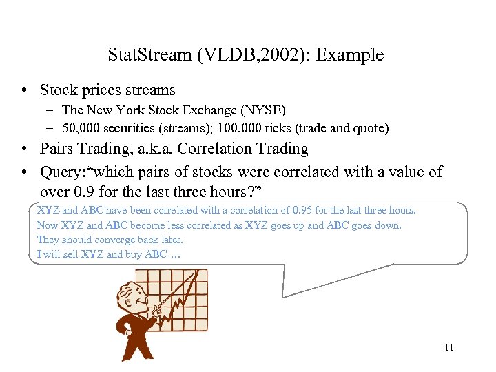Stat. Stream (VLDB, 2002): Example • Stock prices streams – The New York Stock Exchange (NYSE) – 50, 000 securities (streams); 100, 000 ticks (trade and quote) • Pairs Trading, a. k. a. Correlation Trading • Query: “which pairs of stocks were correlated with a value of over 0. 9 for the last three hours? ” XYZ and ABC have been correlated with a correlation of 0. 95 for the last three hours. Now XYZ and ABC become less correlated as XYZ goes up and ABC goes down. They should converge back later. I will sell XYZ and buy ABC … 11

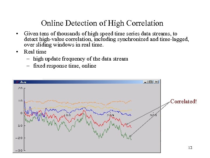Online Detection of High Correlation • Given tens of thousands of high speed time series data streams, to detect high-value correlation, including synchronized and time-lagged, over sliding windows in real time. • Real time – high update frequency of the data stream – fixed response time, online Correlated! 12

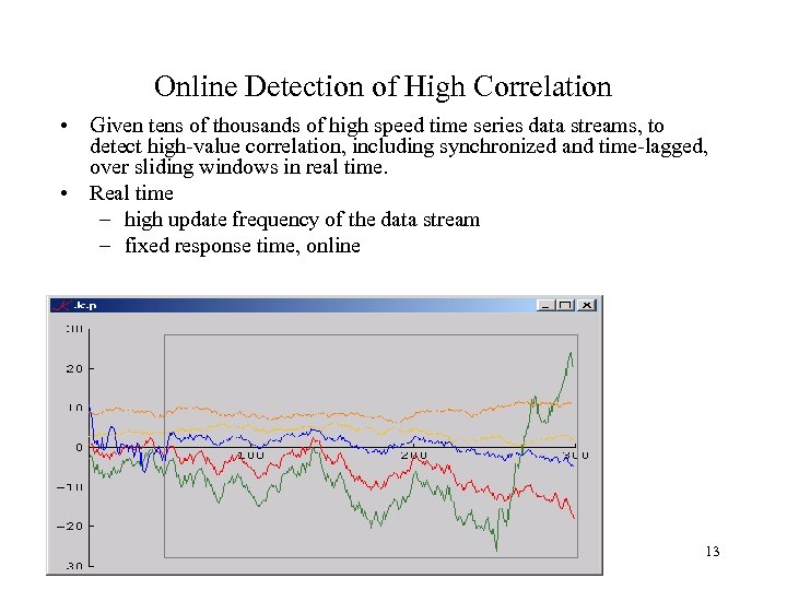Online Detection of High Correlation • Given tens of thousands of high speed time series data streams, to detect high-value correlation, including synchronized and time-lagged, over sliding windows in real time. • Real time – high update frequency of the data stream – fixed response time, online 13

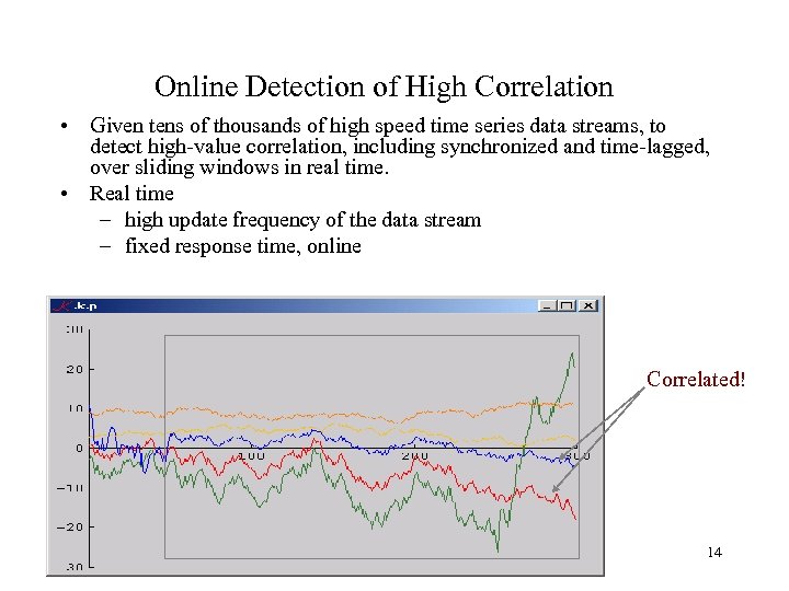Online Detection of High Correlation • Given tens of thousands of high speed time series data streams, to detect high-value correlation, including synchronized and time-lagged, over sliding windows in real time. • Real time – high update frequency of the data stream – fixed response time, online Correlated! 14

Stat. Stream: Naïve Approach • Goal: find most highly correlated stream pairs over sliding windows – N : number of streams – w : size of sliding window – space O(N) and time O(N 2 w). • Suppose that the streams are updated every second. – With a Pentium 4 PC, the exact computing method can monitor only 700 streams, where each result is produced with a separation of two minutes. – Note: “Punctuated result model” – not continuous, but online. 15

Stat. Stream: Our Approach – Use Discrete Fourier Transform to approximate correlation as in Gemini approach. – Every two minutes (“basic window size”), update the DFT for each time series over the last hour (“window size”) – Use grid structure to filter out unlikely pairs – Our approach can report highly correlated pairs among 10, 000 streams for the last hour with a delay of 2 minutes. So, at 2: 02, find highly correlated pairs between 1 PM and 2 PM. At 2: 04, find highly correlated pairs between 1: 02 and 2: 02 PM etc. 16

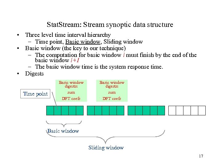Stat. Stream: Stream synoptic data structure • Three level time interval hierarchy – Time point, Basic window, Sliding window • Basic window (the key to our technique) – The computation for basic window i must finish by the end of the basic window i+1 – The basic window time is the system response time. • Digests Time point Basic window digests: sum DFT coefs Basic window Sliding window 17

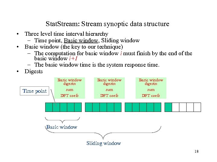Stat. Stream: Stream synoptic data structure • Three level time interval hierarchy – Time point, Basic window, Sliding window • Basic window (the key to our technique) – The computation for basic window i must finish by the end of the basic window i+1 – The basic window time is the system response time. • Digests Time point Basic window digests: sum DFT coefs Basic window Sliding window 18

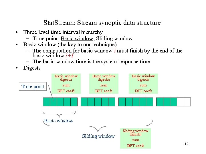Stat. Stream: Stream synoptic data structure • Three level time interval hierarchy – Time point, Basic window, Sliding window • Basic window (the key to our technique) – The computation for basic window i must finish by the end of the basic window i+1 – The basic window time is the system response time. • Digests Time point Basic window digests: sum DFT coefs Basic window Sliding window digests: sum DFT coefs 19

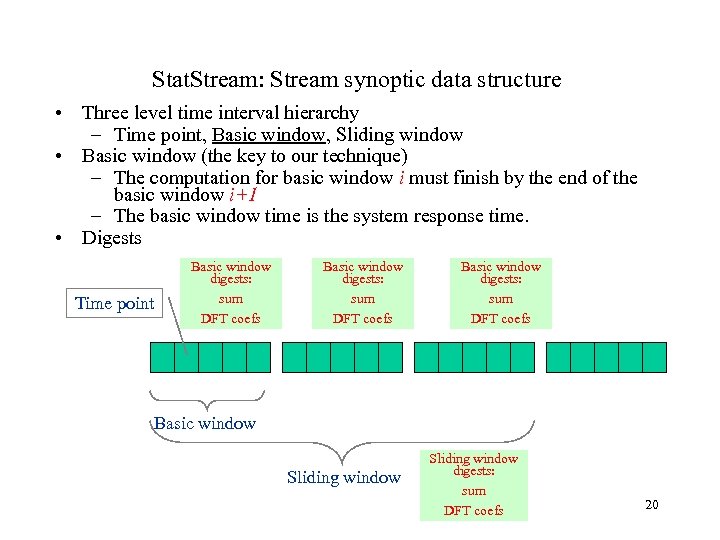Stat. Stream: Stream synoptic data structure • Three level time interval hierarchy – Time point, Basic window, Sliding window • Basic window (the key to our technique) – The computation for basic window i must finish by the end of the basic window i+1 – The basic window time is the system response time. • Digests Time point Basic window digests: sum DFT coefs Basic window Sliding window digests: sum DFT coefs 20

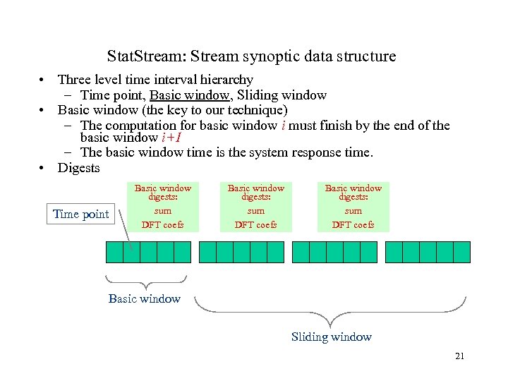Stat. Stream: Stream synoptic data structure • Three level time interval hierarchy – Time point, Basic window, Sliding window • Basic window (the key to our technique) – The computation for basic window i must finish by the end of the basic window i+1 – The basic window time is the system response time. • Digests Time point Basic window digests: sum DFT coefs Basic window Sliding window 21

How general technique is applied • Compress streaming data into moving synopses: Discrete Fourier Transform. • Update the synopses in time proportional to number of coefficients: basic window idea. • Compare synopses in real time: compare DFTs. • Use transforms + simple data structures (grid structure). 22

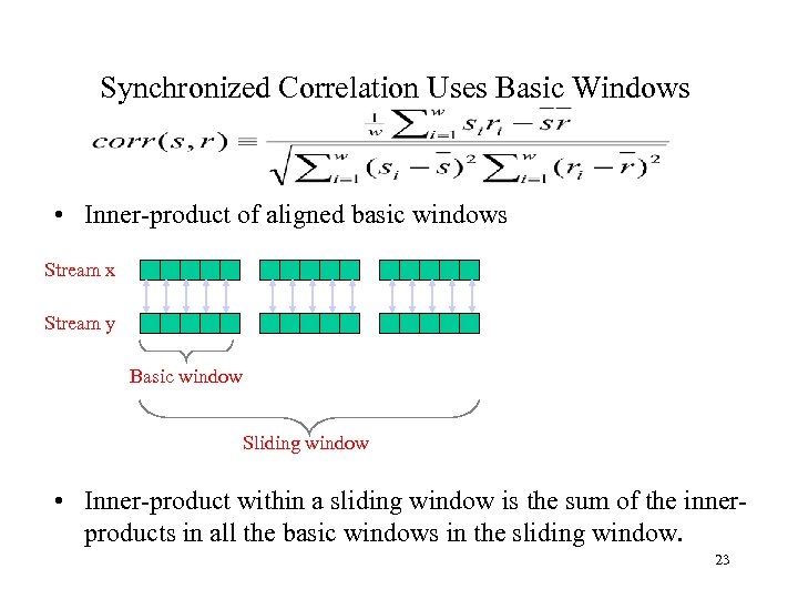Synchronized Correlation Uses Basic Windows • Inner-product of aligned basic windows Stream x Stream y Basic window Sliding window • Inner-product within a sliding window is the sum of the innerproducts in all the basic windows in the sliding window. 23

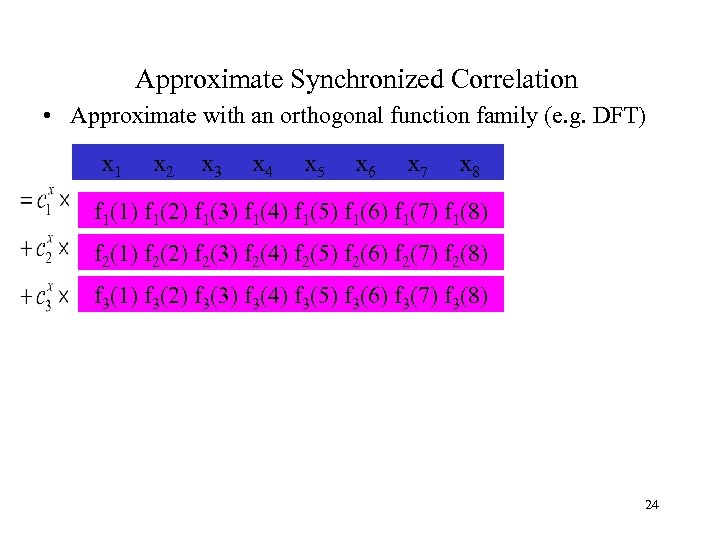Approximate Synchronized Correlation • Approximate with an orthogonal function family (e. g. DFT) x 1 x 2 x 3 x 4 x 5 x 6 x 7 x 8 f 1(1) f 1(2) f 1(3) f 1(4) f 1(5) f 1(6) f 1(7) f 1(8) f 2(1) f 2(2) f 2(3) f 2(4) f 2(5) f 2(6) f 2(7) f 2(8) f 3(1) f 3(2) f 3(3) f 3(4) f 3(5) f 3(6) f 3(7) f 3(8) 24

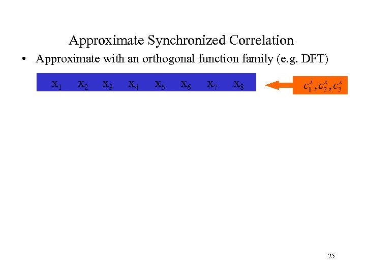Approximate Synchronized Correlation • Approximate with an orthogonal function family (e. g. DFT) x 1 x 2 x 3 x 4 x 5 x 6 x 7 x 8 25

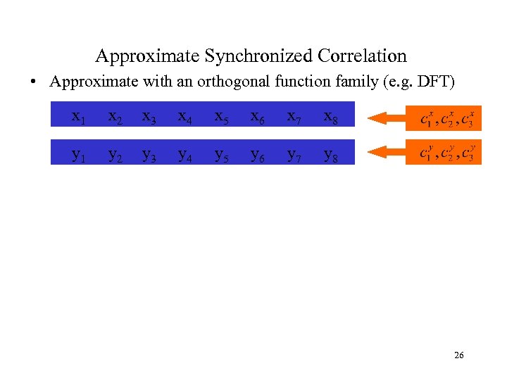Approximate Synchronized Correlation • Approximate with an orthogonal function family (e. g. DFT) x 1 x 2 x 3 x 4 x 5 x 6 x 7 x 8 y 1 y 2 y 3 y 4 y 5 y 6 y 7 y 8 26

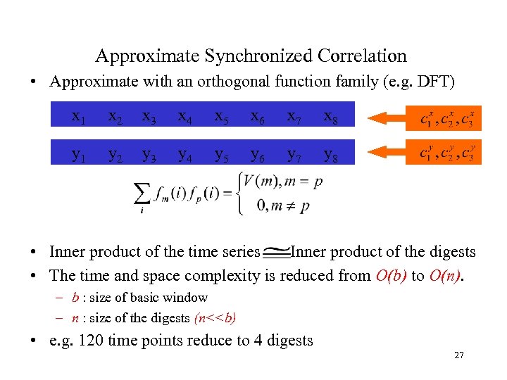Approximate Synchronized Correlation • Approximate with an orthogonal function family (e. g. DFT) x 1 x 2 x 3 x 4 x 5 x 6 x 7 x 8 y 1 y 2 y 3 y 4 y 5 y 6 y 7 y 8 • Inner product of the time series Inner product of the digests • The time and space complexity is reduced from O(b) to O(n). – b : size of basic window – n : size of the digests (n<

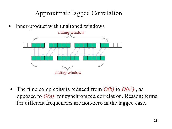Approximate lagged Correlation • Inner-product with unaligned windows sliding window • The time complexity is reduced from O(b) to O(n 2) , as opposed to O(n) for synchronized correlation. Reason: terms for different frequencies are non-zero in the lagged case. 28

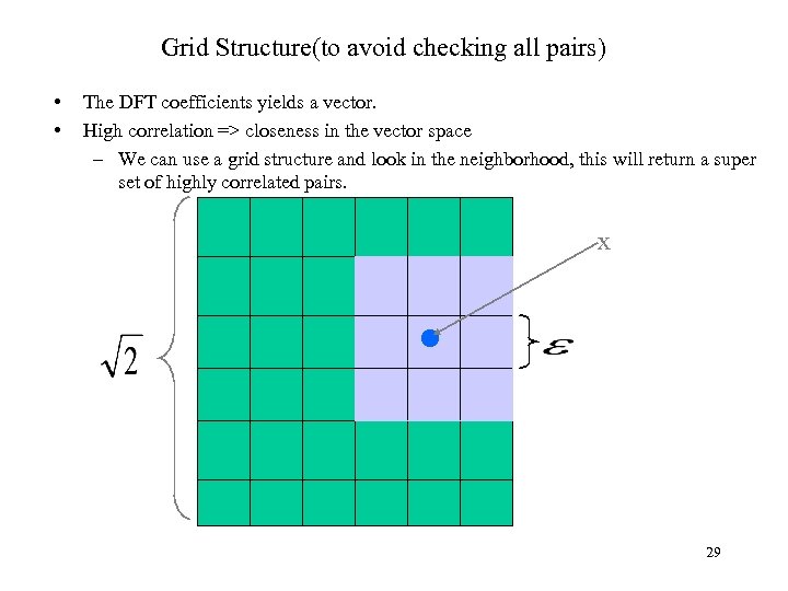Grid Structure(to avoid checking all pairs) • • The DFT coefficients yields a vector. High correlation => closeness in the vector space – We can use a grid structure and look in the neighborhood, this will return a super set of highly correlated pairs. x 29

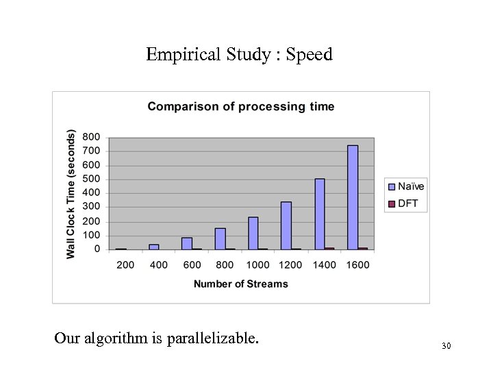Empirical Study : Speed Our algorithm is parallelizable. 30

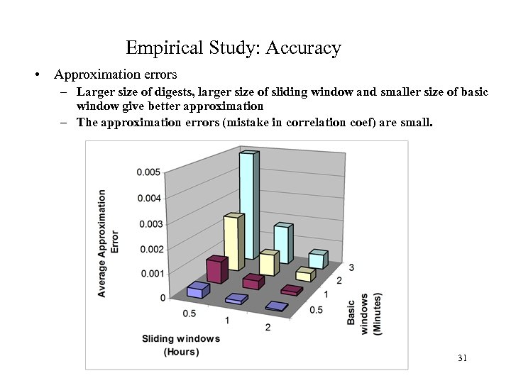Empirical Study: Accuracy • Approximation errors – Larger size of digests, larger size of sliding window and smaller size of basic window give better approximation – The approximation errors (mistake in correlation coef) are small. 31

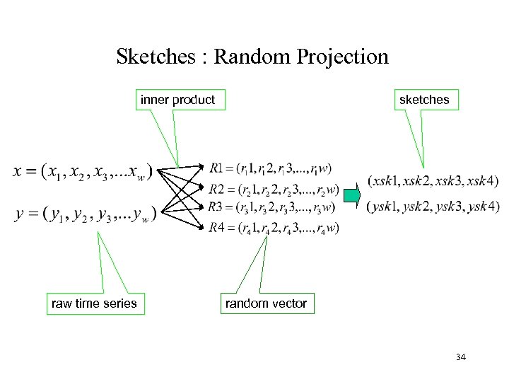
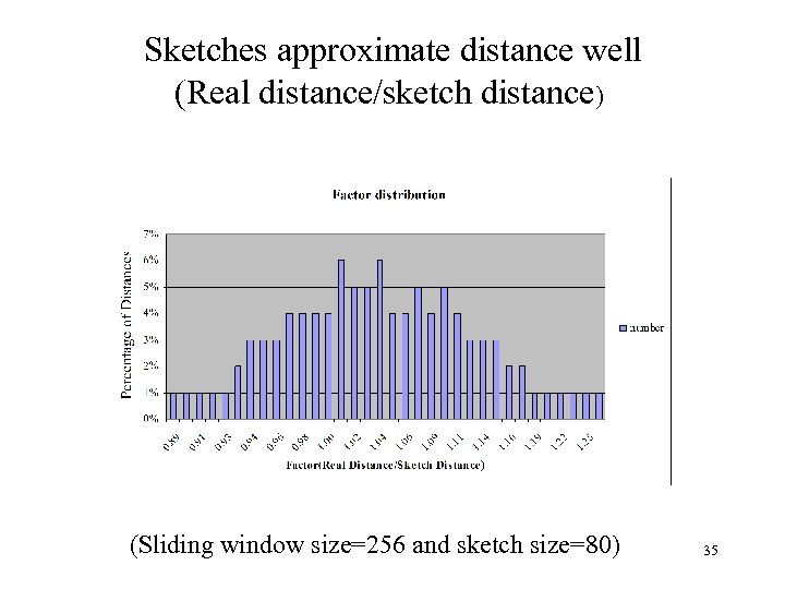
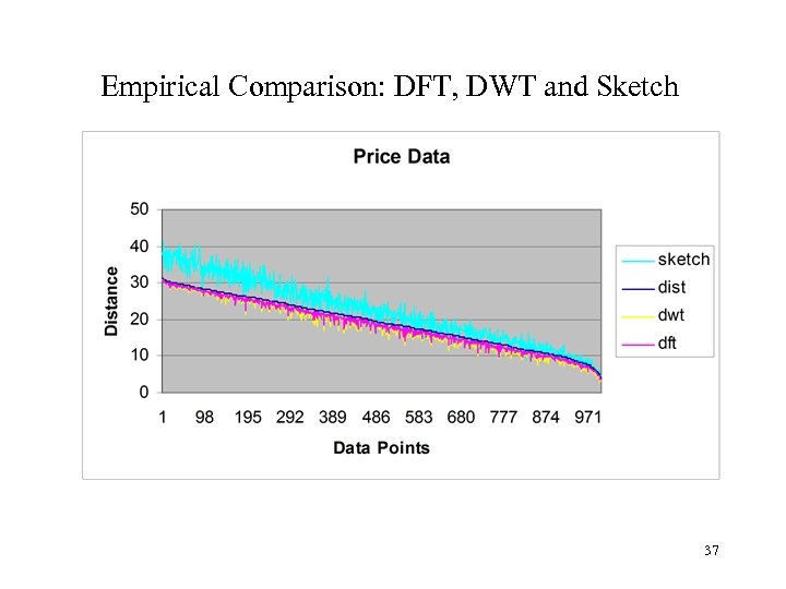
Sketches : Random Projection* • Correlation between time series of the returns of stock – Since most stock price time series are close to random walks, their return time series are close to white noise – DFT/DWT can’t capture approximate white noise series because the energy is distributed across many frequency components. • Solution : Sketches (a form of random landmark) – Sketch pool: list of random vectors drawn from stable distribution – Sketch : The list of inner products from a data vector to the sketch pool. – The Euclidean distance (correlation) between time series is approximated by the distance between their sketches with a probabilistic guarantee. • W. B. Johnson and J. Lindenstrauss. “Extensions of Lipshitz mapping into hilbert space”. Contemp. Math. , 26: 189 -206, 1984 • D. Achlioptas. “Database-friendly random projections”. In Proceedings of the twentieth ACM SIGMOD 32 SIGACT-SIGART symposium on Principles of database systems, ACM Press, 2001

Sketches : Intuition • You are walking in a sparse forest and you are lost. • You have an old-time cell phone without GPS. • You want to know whether you are close to your friend. • You identify yourself as 100 meters from the pointy rock, 200 meters from the giant oak etc. • If your friend is at similar distances from several of these landmarks, you might be close to one another. • The sketch is just the set of distances. 33

Sketches : Random Projection inner product raw time series sketches random vector 34

Sketches approximate distance well (Real distance/sketch distance) (Sliding window size=256 and sketch size=80) 35

Empirical Study: Sketch on Price and Return Data • DFT and DWT work well for prices (today’s price is a good predictor of tomorrow’s) • But badly for returns (todayprice – yesterdayprice)/todayprice. • Data length=256 and the first 14 DFT coefficients are used in the distance computation, db 2 wavelet is used here with coefficient size=16 and sketch size is 64 36

Empirical Comparison: DFT, DWT and Sketch 37

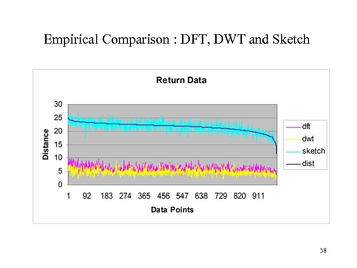Empirical Comparison : DFT, DWT and Sketch 38

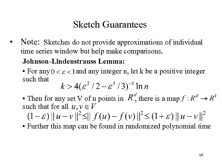Sketch Guarantees • Note: Sketches do not provide approximations of individual time series window but help make comparisons. Johnson-Lindenstrauss Lemma: • For any and any integer n, let k be a positive integer such that • Then for any set V of n points in such that for all , there is a map • Further this map can be found in randomized polynomial time 39

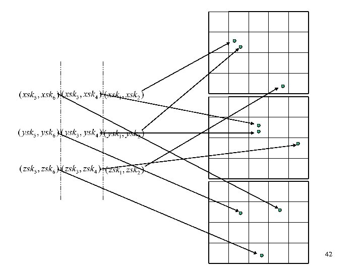
Overcoming curse of dimensionality* • May need many random projections. • Can partition sketches into disjoint pairs or triplets and perform comparisons on those. • Each such small group is placed into an index. • Algorithm must adapt to give the best results. *Idea from P. Indyk, N. Koudas, and S. Muthukrishnan. “Identifying representative trends in massive time series data sets using sketches”. VLDB 2000. 40

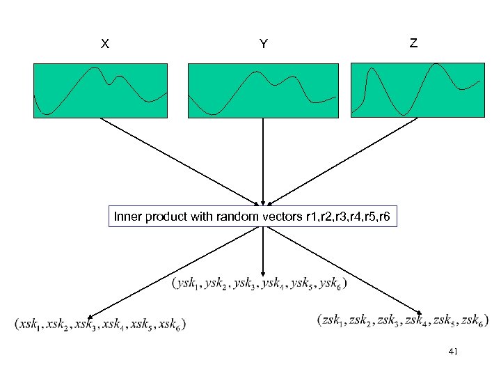X Y Z Inner product with random vectors r 1, r 2, r 3, r 4, r 5, r 6 41

42

Further Performance Improvements -- Suppose we have R random projections of window size WS. -- Might seem that we have to do R*WS work for each timepoint for each time series. -- In ongoing work with colleague Richard Cole, we show that we can cut this down by use of convolution and an oxymoronic notion of “structured random vectors”*. *Idea from Dimitris Achlioptas, “Database-friendly Random Projections”, Proceedings of the twentieth ACM SIGMOD-SIGACT-SIGART symposium on Principles of database systems 43

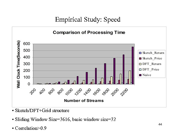Empirical Study: Speed • Sketch/DFT+Grid structure • Sliding Window Size=3616, basic window size=32 • Correlation>0. 9 44

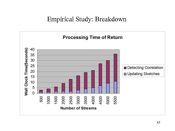Empirical Study: Breakdown 45

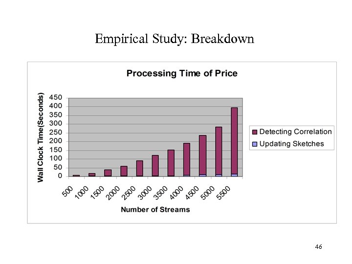Empirical Study: Breakdown 46

Query by humming: Correlation + Shifting

Query By Humming • You have a song in your head. • You want to get it but don’t know its title. • If you’re not too shy, you hum it to your friends or to a salesperson and you find it. • They may grimace, but you get your CD 48

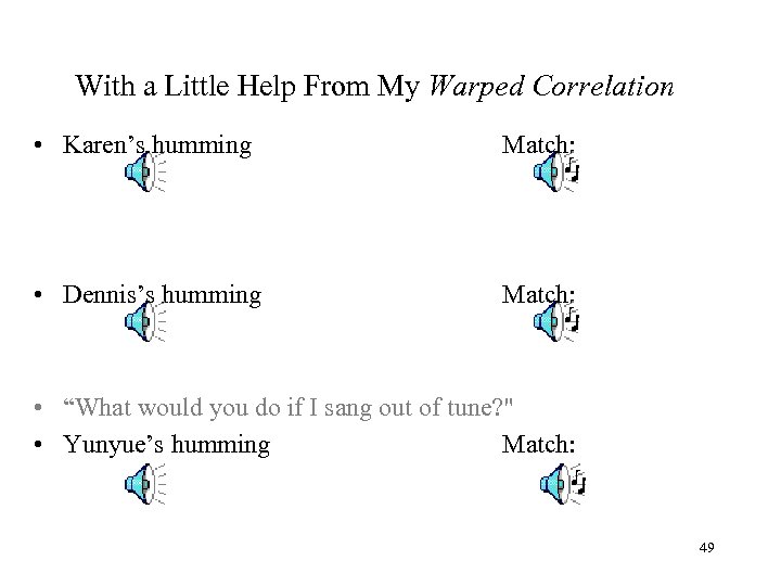With a Little Help From My Warped Correlation • Karen’s humming Match: • Dennis’s humming Match: • “What would you do if I sang out of tune? " • Yunyue’s humming Match: 49

Related Work in Query by Humming • Traditional method: String Matching [Ghias et. al. 95, Mc. Nab et. al. 97, Uitdenbgerd and Zobel 99] – Music represented by string of pitch directions: U, D, S (degenerated interval) – Hum query is segmented to discrete notes, then string of pitch directions – Edit Distance between hum query and music score • Problem – Very hard to segment the hum query – Partial solution: users are asked to hum articulately • New Method : matching directly from audio [Mazzoni and Dannenberg 00] • We use both. 50

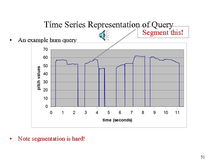Time Series Representation of Query • An example hum query Segment this! • Note segmentation is hard! 51

How to deal with poor hummers? • No absolute pitch – Solution: the average pitch is subtracted • Inaccurate pitch intervals – Solution: return the k-nearest neighbors • Incorrect overall tempo – Solution: Uniform Time Warping • Local timing variations – Solution: Dynamic Time Warping • Bottom line: timing variations take us beyond Euclidean distance. 52

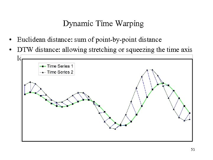Dynamic Time Warping • Euclidean distance: sum of point-by-point distance • DTW distance: allowing stretching or squeezing the time axis locally 53

Envelope Transform using Piecewise Aggregate Approximation(PAA) [Keogh VLDB 02] 54

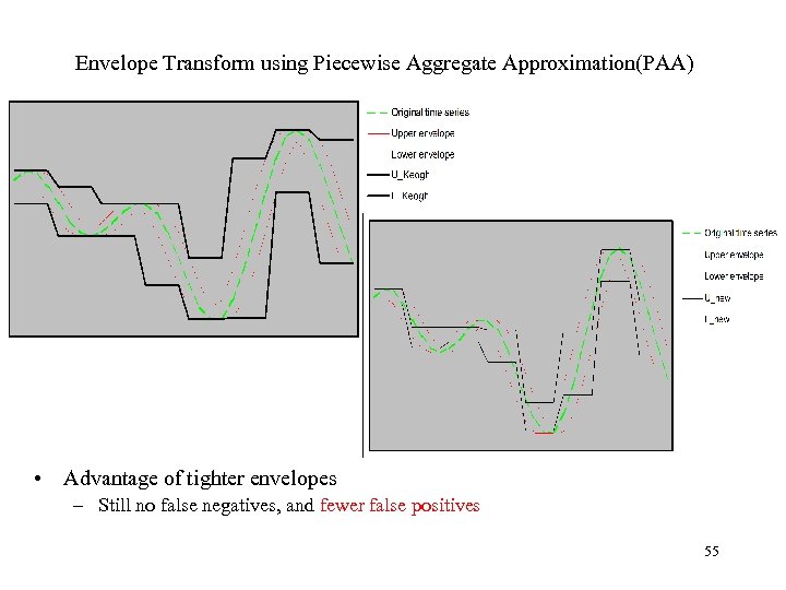Envelope Transform using Piecewise Aggregate Approximation(PAA) • Advantage of tighter envelopes – Still no false negatives, and fewer false positives 55

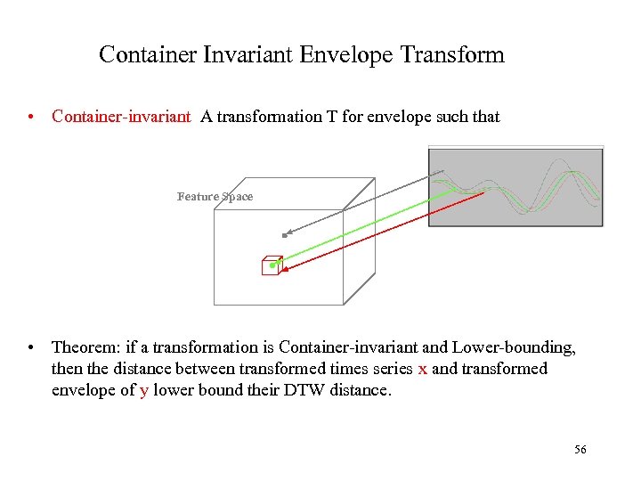Container Invariant Envelope Transform • Container-invariant A transformation T for envelope such that Feature Space • Theorem: if a transformation is Container-invariant and Lower-bounding, then the distance between transformed times series x and transformed envelope of y lower bound their DTW distance. 56

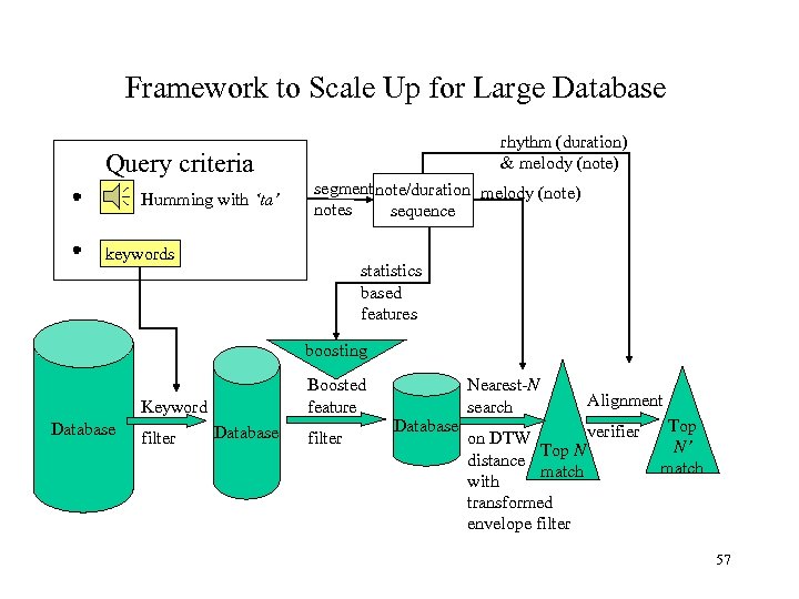Framework to Scale Up for Large Database rhythm (duration) & melody (note) Query criteria Humming with ‘ta’ segment note/duration melody (note) notes sequence keywords statistics based features boosting Boosted feature Keyword Database filter Database Nearest-N search Alignment verifier on DTW Top N distance match with transformed envelope filter Top N’ match 57

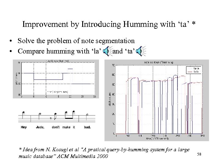Improvement by Introducing Humming with ‘ta’ * • Solve the problem of note segmentation • Compare humming with ‘la’ and ‘ta’ * Idea from N. Kosugi et al “A pratical query-by-humming system for a large music database” ACM Multimedia 2000 58

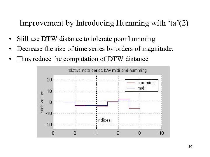Improvement by Introducing Humming with ‘ta’(2) • Still use DTW distance to tolerate poor humming • Decrease the size of time series by orders of magnitude. • Thus reduce the computation of DTW distance 59

Statistics-Based Filters * • Low dimensional statistic feature comparison – Low computation cost comparing to DTW distance – Quickly filter out true negatives • Example – Filter out candidates whose note length is much larger/smaller than the query’s note length • More – – Standard Derivation of note value Zero crossing rate of note value Number of local minima of note value Number of local maxima of note value * Intuition from Erling Wold et al “Content-based classification, search and retrieval of audio” IEEE Multimedia 1996 http: //www. musclefish. com 60

Boosting Statistics-Based Filters • Characteristics of statistics-based filters – Quick but weak classifier – May have false negatives/false positives – Ideal candidates for boosting • Boosting * – “An algorithm for constructing a ‘strong’ classifier using only a training set and a set of ‘weak’ classification algorithm” – “A particular linear combination of these weak classifiers is used as the final classifier which has a much smaller probability of misclassification” * Cynthia Rudin et al “On the Dynamics of Boosting” In Advances in Neural Information Processing Systems 2004 61

Verify Rhythm Alignment in the Query Result • • Nearest-N search only used melody information Will A. Arentz et al* suggests combining rhythm and melody – Results are generally better than using only melody information – Not appropriate when the sum of several notes’ duration in the query may be related to duration of one note in the candidate • Our method: – First use melody information for DTW distance computing – Merge durations appropriately based on the note alignment – Reject candidates which have bad rhythm alignment * Will Archer Arentz “Methods for retrieving musical information based on rhythm and pitch correlation” CSGSC 2003 62

Experiments: Setup • Data Set – – • Query Algorithms Comparison – – – • TS: matching pitch-contour time series using DTW distance and envelope filters NS: matching ‘ta’-based note-sequence using DTW distance and envelope filters plus length and standard-derivation based filters NS 2: NS plus boosted statistics-based filters and alignment verifiers Training Set: Human humming query set – – – • 1049 songs: Beatles, American Rock and Pop, one Chinese song 73, 051 song segments 17 ‘ta’-style humming clips from 13 songs (half are Beatles songs) The number of notes varies from 8 to 25, average 15 The matching song segments are labeled by musicians Test Set: Simulated queries – – Queries are generated based on 1000 randomly selected segments in database The following error types are simulated: different keys/tempos, inaccurate pitch intervals, varying tempos, missing/extra notes and background noise * * The error model is experimental and the error parameters are based on the analysis of training set 63

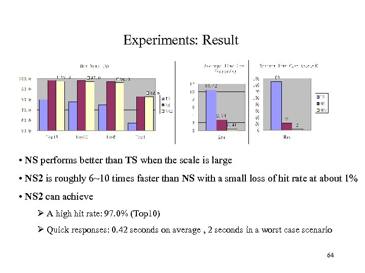Experiments: Result • NS performs better than TS when the scale is large • NS 2 is roughly 6~10 times faster than NS with a small loss of hit rate at about 1% • NS 2 can achieve Ø A high hit rate: 97. 0% (Top 10) Ø Quick responses: 0. 42 seconds on average , 2 seconds in a worst case scenario 64

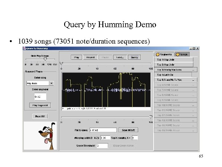Query by Humming Demo • 1039 songs (73051 note/duration sequences) 65

Burst detection: when window size is unknown

Burst Detection: Applications • Discovering intervals with unusually large numbers of events. – In astrophysics, the sky is constantly observed for high-energy particles. When a particular astrophysical event happens, a shower of high-energy particles arrives in addition to the background noise. Might last milliseconds or days… – In telecommunications, if the number of packages lost within a certain time period exceeds some threshold, it might indicate some network anomaly. Exact duration is unknown. – In finance, stocks with unusual high trading volumes should attract the notice of traders (or perhaps regulators). 67

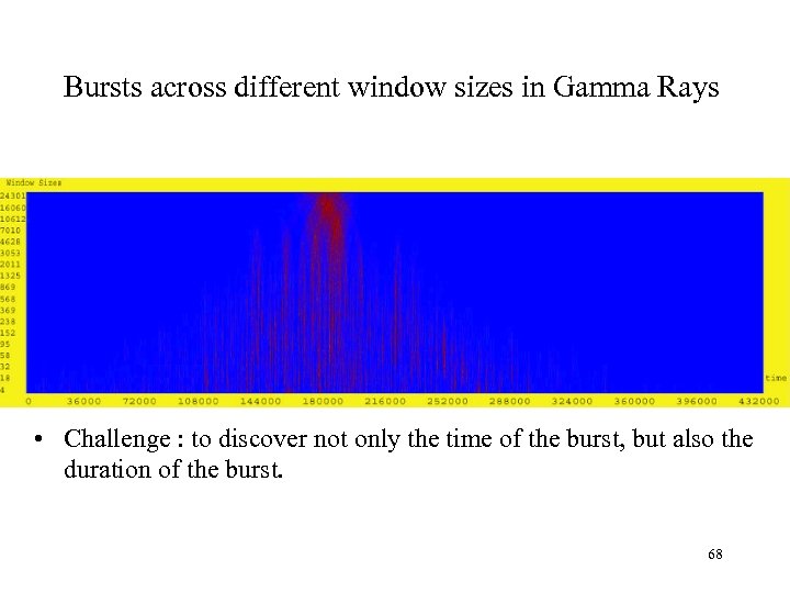Bursts across different window sizes in Gamma Rays • Challenge : to discover not only the time of the burst, but also the duration of the burst. 68

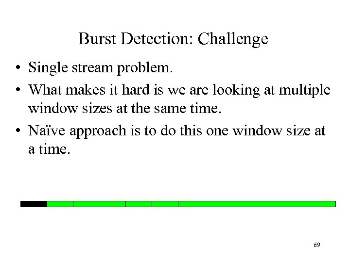Burst Detection: Challenge • Single stream problem. • What makes it hard is we are looking at multiple window sizes at the same time. • Naïve approach is to do this one window size at a time. 69

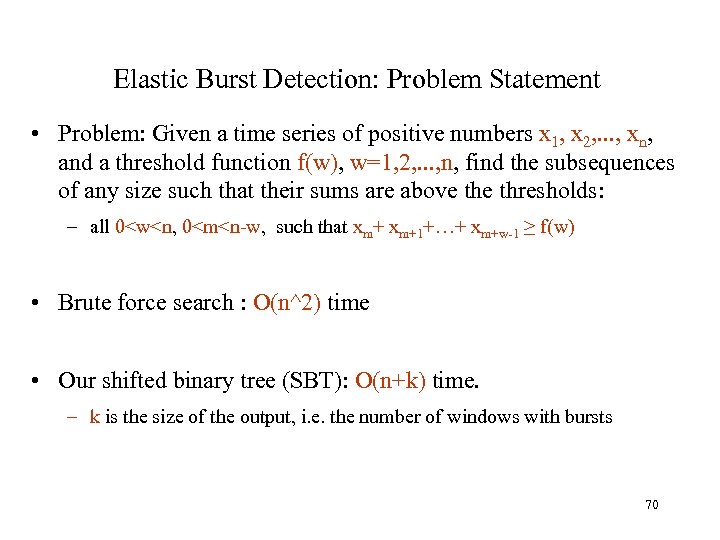Elastic Burst Detection: Problem Statement • Problem: Given a time series of positive numbers x 1, x 2, . . . , xn, and a threshold function f(w), w=1, 2, . . . , n, find the subsequences of any size such that their sums are above thresholds: – all 0

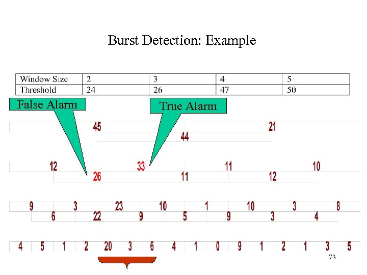
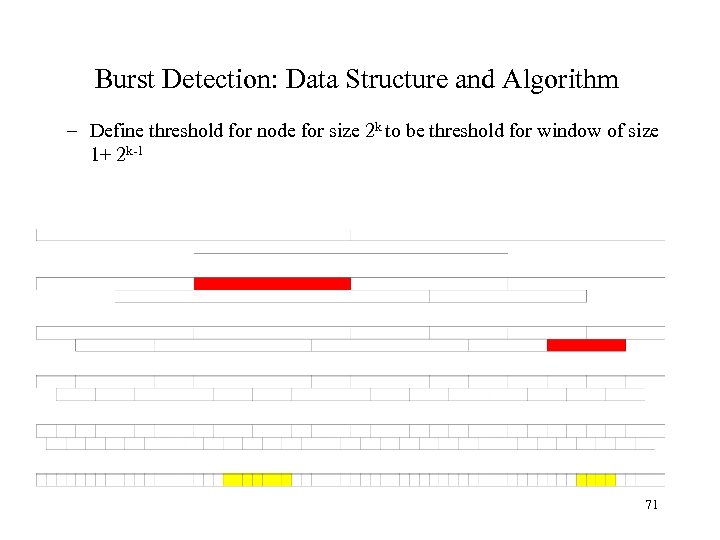Burst Detection: Data Structure and Algorithm – Define threshold for node for size 2 k to be threshold for window of size 1+ 2 k-1 71

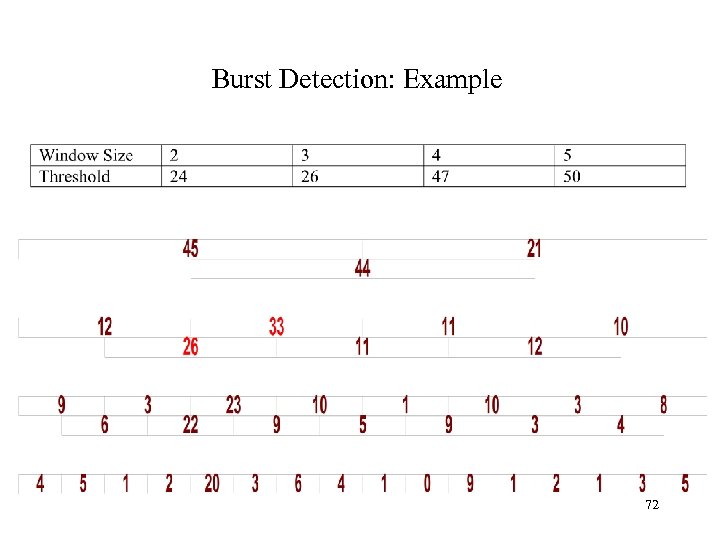Burst Detection: Example 72

Burst Detection: Example False Alarm True Alarm 73

Burst Detection: Algorithm • In linear time, determine whether any node in SBT indicates an alarm. • If so, do a detailed search to confirm (true alarm) or deny (false alarm) a real burst. • In on-line version of the algorithm, need keep only most recent node at each level. 74

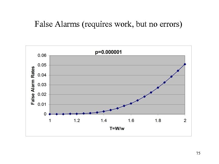False Alarms (requires work, but no errors) 75

Empirical Study : Gamma Ray Burst 76

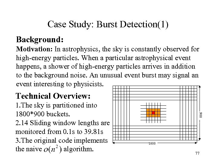Case Study: Burst Detection(1) Background: Motivation: In astrophysics, the sky is constantly observed for high-energy particles. When a particular astrophysical event happens, a shower of high-energy particles arrives in addition to the background noise. An unusual event burst may signal an event interesting to physicists. Technical Overview: 900 1. The sky is partitioned into 1800*900 buckets. 2. 14 Sliding window lengths are monitored from 0. 1 s to 39. 81 s 3. The original code implements the naive algorithm. 1800 77

Case Study: Burst Detection(2) The challenges: 1. Vast amount of data § 1800*900 time series, so any trivial overhead may be accumulated to become a nontrivial expense. 2. Unavoidable overheads of data transformations § § Data pre-processing such as fetching and storage requires much work. SBT trees have to be built no matter how many sliding windows to be investigated. § Thresholds are maintained over time due to the different background noises. § Hit on one bucket will affect its neighbours as shown in the previous figure 78

Case Study: Burst Detection(3) Our solutions: 1. Combine near buckets into one to save space and processing time. If any alarms reported for this large bucket, go down to see each small components (two level detailed search). 2. Special implementation of SBT tree § Build the SBT tree only including those levels covering the sliding windows § Maintain a threshold tree for the sliding windows and update it over time. Fringe benefits: 1. Adding window sizes is easy. 2. More sliding windows monitored also benefit physicists. 79

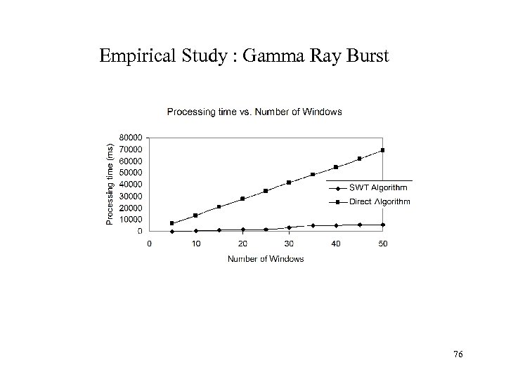
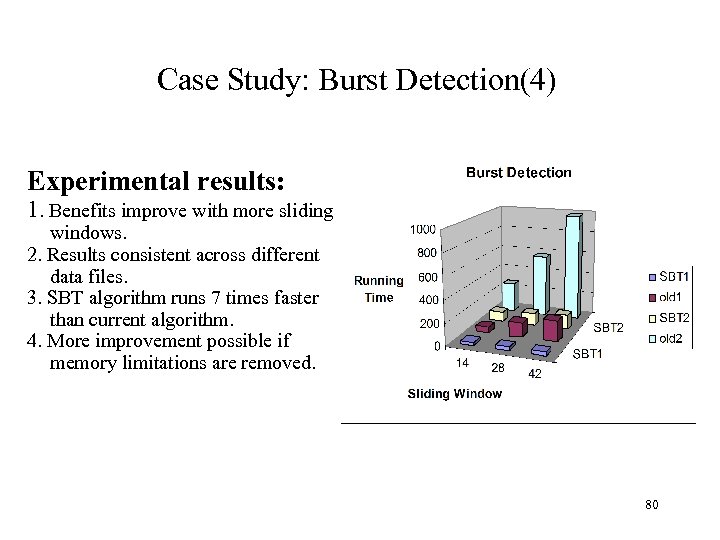Case Study: Burst Detection(4) Experimental results: 1. Benefits improve with more sliding windows. 2. Results consistent across different data files. 3. SBT algorithm runs 7 times faster than current algorithm. 4. More improvement possible if memory limitations are removed. 80

Extension to other aggregates • SBT can be used for any aggregate that is monotonic – SUM, COUNT and MAX are monotonically increasing • the alarm threshold is aggregate

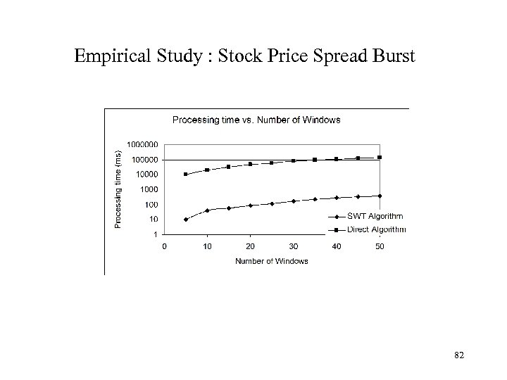Empirical Study : Stock Price Spread Burst 82

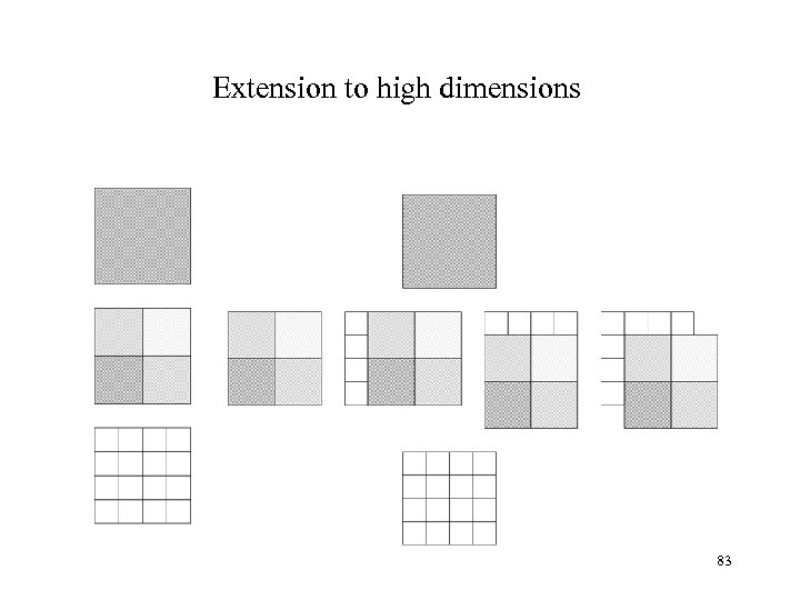Extension to high dimensions 83

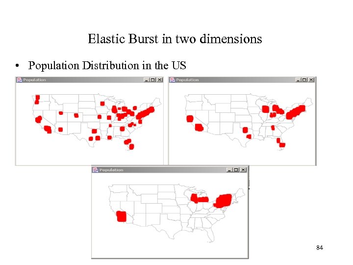Elastic Burst in two dimensions • Population Distribution in the US 84

Can discover numeric thresholds from probability threshold. • Suppose that the moving sum of a time series is a random variable from a normal distribution. • Let the number of bursts in the time series within sliding window size w be So(w) and its expectation be Se(w). – Se(w) can be computed from the historical data. • Given a threshold probability p, we set the threshold of burst f(w) for window size w such that Pr[So(w) ≥ f(w)] ≤p. 85

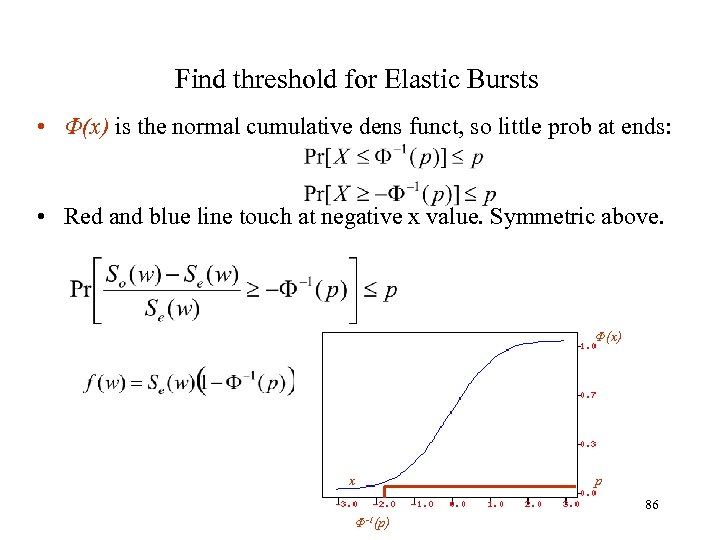Find threshold for Elastic Bursts • Φ(x) is the normal cumulative dens funct, so little prob at ends: • Red and blue line touch at negative x value. Symmetric above. Φ(x) x p 86 Φ-1(p)

Summary of Burst Detection • Able to detect bursts on many different window sizes in essentially linear time. • Can be used both for time series and for spatial searching. • Can specify thresholds either with absolute numbers or with probability of hit. • Algorithm is simple to implement and has low constants (code is available). • Ok, it’s embarrassingly simple. 87

AQuery A Database System for Order

Time Series and DBMS’s • Usual approach is to store time series as a User Defined Datatype (UDT) and provide methods for manipulating it • Advantages – series can be stored and manipulated by DBMS • Disadvantages – UDTs are somewhat opaque to the optimizer (it misses opportunities) – Operations that mix series and “regular” data may be awkward to write 89

The Case for Order 1 • Series are sequences! Support them. • Add order to multiset-based DBMS 2, 3, 4 • AQuery is a query language (conservative SQL extension) and a data model that supports order from the ground up “A Call to Order”, David Maier and Bennet Vance, PODS’ 93 2 “SRQL: Sorted Relational Query Language”, Ramakrishnan et al. , SSDBM’ 98 3 “SEQ: A Model for Sequence Databases”, Seshadri et al. , ICDE’ 95 4 OLAP Amendment to SQL: 1999 1 90

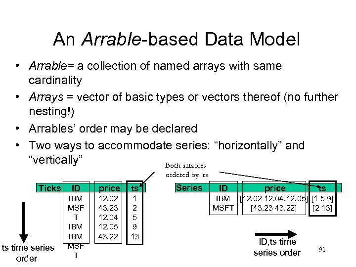An Arrable-based Data Model • Arrable= a collection of named arrays with same cardinality • Arrays = vector of basic types or vectors thereof (no further nesting!) • Arrables’ order may be declared • Two ways to accommodate series: “horizontally” and “vertically” Both arrables ordered by ts Ticks ts time series order ID price ts IBM MSF T 12. 02 43. 23 12. 04 12. 05 43. 22 1 2 5 9 13 Series ID price ts IBM [12. 02 12. 04. 12. 05] [1 5 9] MSFT [43. 23 43. 22] [2 13] ID, ts time series order 91

AQuery’s New Language Elements • ASSUMING ORDER clause – Order is explicitly declared on a per-query basis – All other clauses can count on order (and preserve it) • Column-Oriented Semantics – AQuery: R. col in a query binds to an array/vector (an entire column) – SQL: R. col binds successively to the scalar field values in a column • Built-in functions for order-dependent aggs over columns • Can group by without aggregation 92

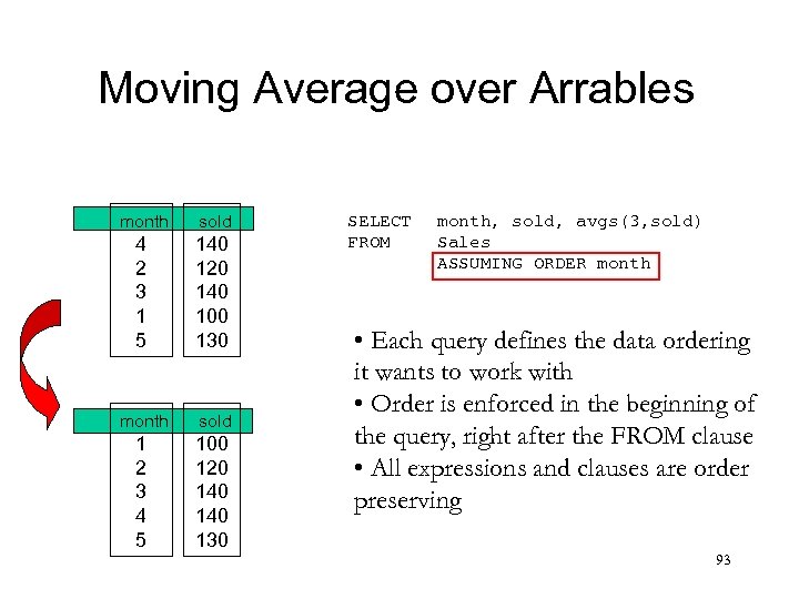Moving Average over Arrables month sold 4 2 3 1 5 140 120 140 100 130 month sold 1 2 3 4 5 100 120 140 130 SELECT FROM month, sold, avgs(3, sold) Sales ASSUMING ORDER month • Each query defines the data ordering it wants to work with • Order is enforced in the beginning of the query, right after the FROM clause • All expressions and clauses are order preserving 93

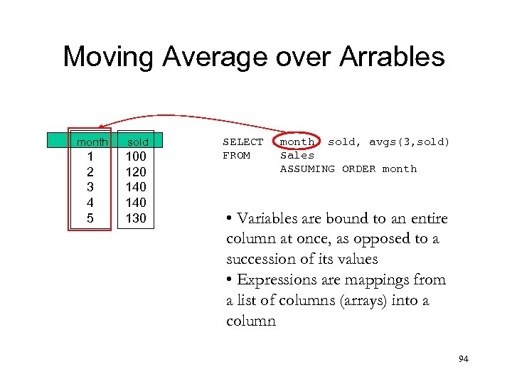Moving Average over Arrables month sold 1 2 3 4 5 100 120 140 130 SELECT FROM month, sold, avgs(3, sold) Sales ASSUMING ORDER month • Variables are bound to an entire column at once, as opposed to a succession of its values • Expressions are mappings from a list of columns (arrays) into a column 94

Moving Average over Arrables month sold 3 -avg 1 2 3 4 5 100 120 140 130 100 110 120 133 136 SELECT FROM month, sold, avgs(3, sold) Sales ASSUMING ORDER month • Several built in “vector-to-vector” functions • Avgs, for instance, takes a window size and a column and returns the resulting moving average column • Other v 2 v functions: prev, next, first, last, sums, mins, . . . , and UDFs 95

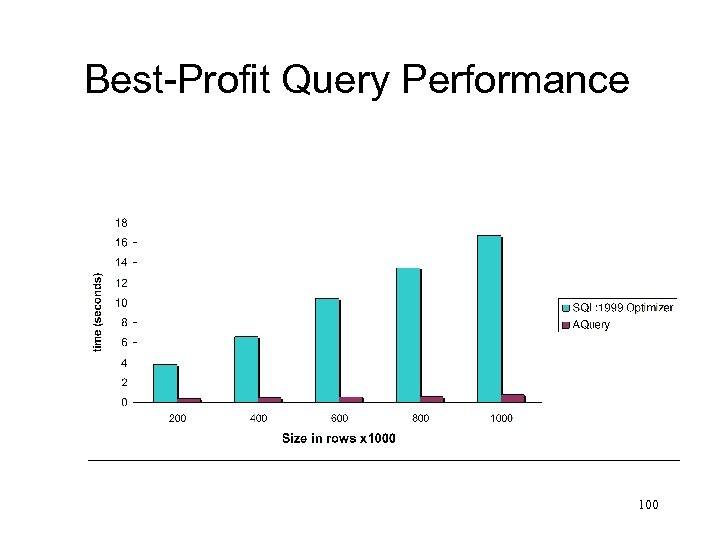
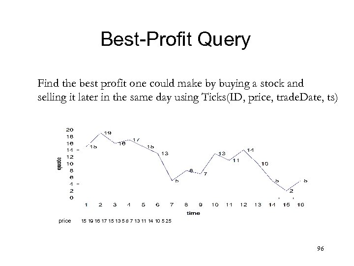Best-Profit Query Find the best profit one could make by buying a stock and selling it later in the same day using Ticks(ID, price, trade. Date, ts) price 15 19 16 17 15 13 5 8 7 13 11 14 10 5 2 5 96

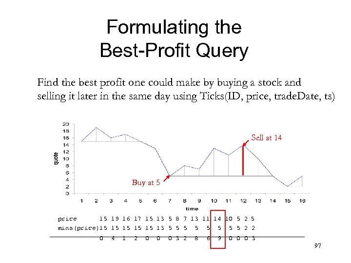Formulating the Best-Profit Query Find the best profit one could make by buying a stock and selling it later in the same day using Ticks(ID, price, trade. Date, ts) Sell at 14 Buy at 5 price 15 19 16 17 15 13 5 8 7 13 11 14 10 5 2 5 mins(price)15 15 15 13 5 5 5 5 2 2 0 4 1 2 0 0 0 3 2 8 6 9 0 0 0 3 97

Best-Profit Query Comparison [AQuery] SELECT max(price–mins(price)) FROM ticks ASSUMING timestamp WHERE ID=“S” AND trade. Date=‘ 1/10/03' [SQL: 1999] SELECT max(rdif) FROM (SELECT ID, trade. Date, price - min(price) OVER (PARTITION BY ID, trade. Date ORDER BY timestamp ROWS UNBOUNDED PRECEDING) AS rdif FROM Ticks ) AS t 1 WHERE ID=“S” AND trade. Date=‘ 1/10/03' 98

Best-Profit Query Comparison [AQuery] SELECT max(price–mins(price)) FROM ticks ASSUMING timestamp WHERE ID=“S” AND trade. Date=‘ 1/10/03' [SQL: 1999] SELECT max(rdif) FROM (SELECT ID, trade. Date, price - min(price) OVER (PARTITION BY ID, trade. Date ORDER BY timestamp ROWS UNBOUNDED PRECEDING) AS rdif FROM Ticks ) AS t 1 WHERE ID=“S” AND trade. Date=‘ 1/10/03' AQuery optimizer can push down the selection simply by testing whether selection is order dependent or not; SQL: 1999 optimizer has to figure out if the selection would alter semantics of the windows (partition), a much harder question. 99

Best-Profit Query Performance 100

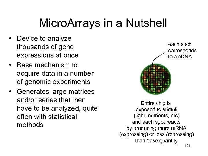Micro. Arrays in a Nutshell • Device to analyze thousands of gene expressions at once • Base mechanism to acquire data in a number of genomic experiments • Generates large matrices and/or series that then have to be analyzed, quite often with statistical methods each spot corresponds to a c. DNA Entire chip is exposed to stimuli (light, nutrients, etc) and each spot reacts by producing more m. RNA (expressing) or less (repressing) than base quantity 101

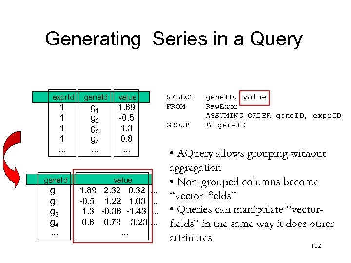Generating Series in a Query expr. Id gene. Id value 1 1. . . g 1 g 2 g 3 g 4. . . 1. 89 -0. 5 1. 3 0. 8. . . gene. Id g 1 g 2 g 3 g 4. . . value 1. 89 -0. 5 1. 3 0. 8 2. 32 0. 32. . . 1. 22 1. 03. . . -0. 38 -1. 43. . . 0. 79 3. 23. . . SELECT FROM GROUP gene. ID, value Raw. Expr ASSUMING ORDER gene. ID, expr. ID BY gene. ID • AQuery allows grouping without aggregation • Non-grouped columns become “vector-fields” • Queries can manipulate “vectorfields” in the same way it does other attributes 102

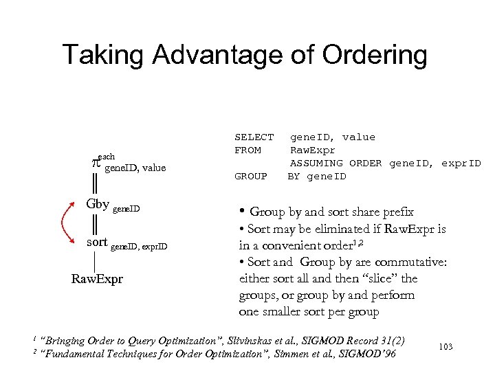Taking Advantage of Ordering each gene. ID, value Gby gene. ID sort gene. ID, expr. ID Raw. Expr 1 2 SELECT FROM GROUP gene. ID, value Raw. Expr ASSUMING ORDER gene. ID, expr. ID BY gene. ID • Group by and sort share prefix • Sort may be eliminated if Raw. Expr is in a convenient order 1, 2 • Sort and Group by are commutative: either sort all and then “slice” the groups, or group by and perform one smaller sort per group “Bringing Order to Query Optimization”, Slivinskas et al. , SIGMOD Record 31(2) “Fundamental Techniques for Order Optimization”, Simmen et al. , SIGMOD’ 96 103

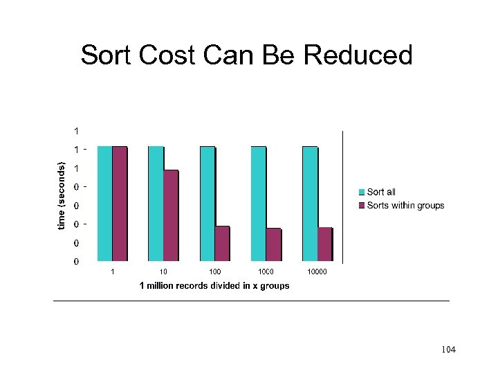Sort Cost Can Be Reduced 104

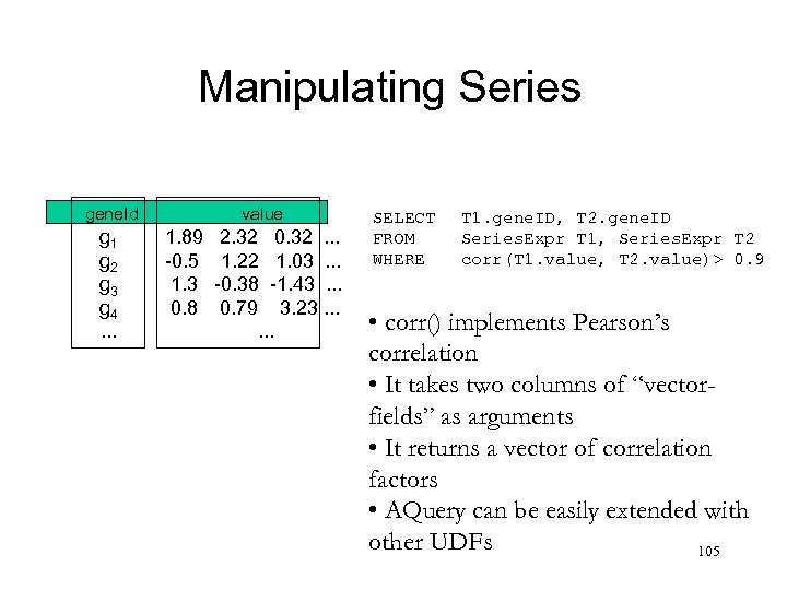Manipulating Series gene. Id g 1 g 2 g 3 g 4. . . value 1. 89 -0. 5 1. 3 0. 8 2. 32 0. 32. . . 1. 22 1. 03. . . -0. 38 -1. 43. . . 0. 79 3. 23. . . SELECT FROM WHERE T 1. gene. ID, T 2. gene. ID Series. Expr T 1, Series. Expr T 2 corr(T 1. value, T 2. value)> 0. 9 • corr() implements Pearson’s correlation • It takes two columns of “vectorfields” as arguments • It returns a vector of correlation factors • AQuery can be easily extended with other UDFs 105

AQuery Summary • AQuery is a natural evolution from the Relational Model • AQuery is a concise language for querying order • Optimization possibilities are vast • Applications to Finance, Physics, Biology, Network Management, . . . 106

Overall Summary • Improved technology implies better sensors and more data. • Real-time response is very useful and profitable in applications ranging from astrophysics to finance. • These require better algorithms and better data management. • This is a great field for research and teaching. 107