Faculty of Social Sciences Induction Block Maths

Faculty of Social Sciences Induction Block: Maths & Statistics Lecture 6: Sample size, SPSS and Hypothesis Testing Dr Gwilym Pryce 1

Plan n n 1. Summary of L 5 2. Statistical Significance 3. Type 1 and Type II errors 4. Four steps of Hypothesis Testing 5. Overview of the Course 2

1. Summary of L 5: n n Social Research is usually based on samples We usually want to use our sample to say something about the population – I. e. we want to be able to generalise n n How precisely we can estimate the population mean or proportion depends on our sample size and the variation within the sample Using the CLT, statistical inference offers a systematic way of establishing: – the range of values in which the population mean or proportion is likely to lie (‘a confidence interval’). – Whether a hypothesis about a mean or a 3 proportion is likely to hold in the population.

2. Statistical Significance n “Significance” does not refer to “importance” – but to “real differences in fact” between our observed sample mean and our assumption about the population mean n P = significance level = chances of our observed sample mean occurring given that our assumption about the population (denoted by “H 0”) is true. – So if we find that this probability is small, it might lead us to question our assumption about the population mean. 4

n I. e. if our sample mean is a long way from our assumed population mean then it is: – either a freak sample – or our assumption about the population mean is wrong. n If we draw the conclusion that it is our assumption that is wrong and reject H 0 then we have to bear in mind that there is a chance that H 0 was in fact true. – I. e. every twenty times we reject H 0 when P = 0. 05, then on one of those occasions we would have rejected H 0 when it was in fact true. 5

n n Obviously, as the sample mean moves further away from our assumption (H 0) about the population mean, we have stronger evidence that H 0 is false. If P is very small, say 0. 001, then there is only 1 chance in a thousand of our observed sample mean occurring if H 0 is true. – This also means that if we reject H 0 when P = 0. 001, then there is only one in a thousand chance that we have made a mistake (I. e. that we have been guilty of a “Type I error”) 6

n There is a tradition (initiated by English scientist R. A. Fisher 1860 -1962) of rejecting H 0 if the probability of incorrectly rejecting it is 0. 05. – If P 0. 05 then we say that H 0 can be rejected at the 5% significance level. – If P > 0. 05, then, argued Fisher, the chances of incorrectly rejecting H 0 are too high to allow us to do so. n Sig level = P = the probability of a sample mean at least as extreme as our observed value occurring, given our assumption about the population mean. 7

3. Type I and Type II errors: n P = significance level = chances of incorrectly rejecting H 0 when it is in fact true. – Called a “Type I error” n If we accept H 0 when in fact the alternative hypothesis is true – Called a “Type II error”. n On this course we shall be concerned only with Type I errors. 8

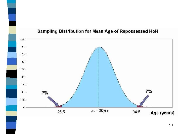
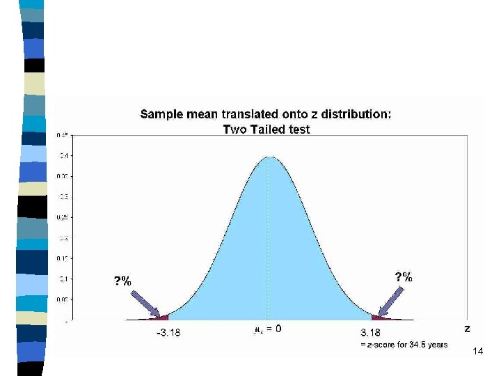
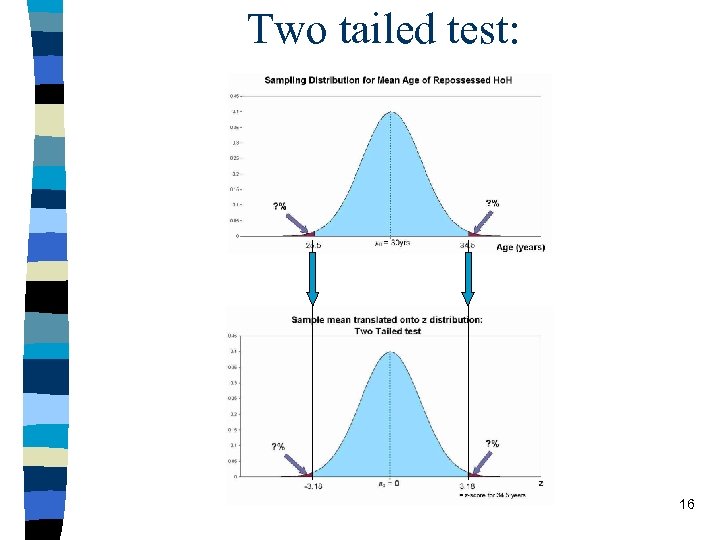
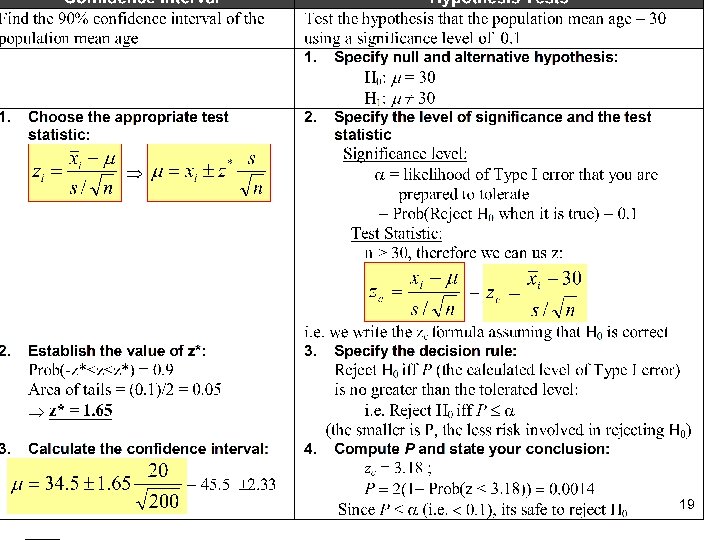
4. The four steps of hypothesis testing n Last lecture we looked at confidence intervals: – establish the range of values of the population mean for a given level of confidence • e. g. we are 90% confident that population mean age of Ho. Hs in repossessed dwellings in the Great Depression lay between 32. 17 and 36. 83 years (s = 20). • Based on a sample of 200 with mean = 34. 5 yrs. – But what if we want to use our sample to test a specific hypothesis we may have about the population mean? • E. g. does m = 30 years? – If m does = 30 years, then how likely are we to select a sample with a mean as extreme as 34. 5 years? » I. e. 4. 5 years more or 4. 5 years less than the pop mean? 9

10

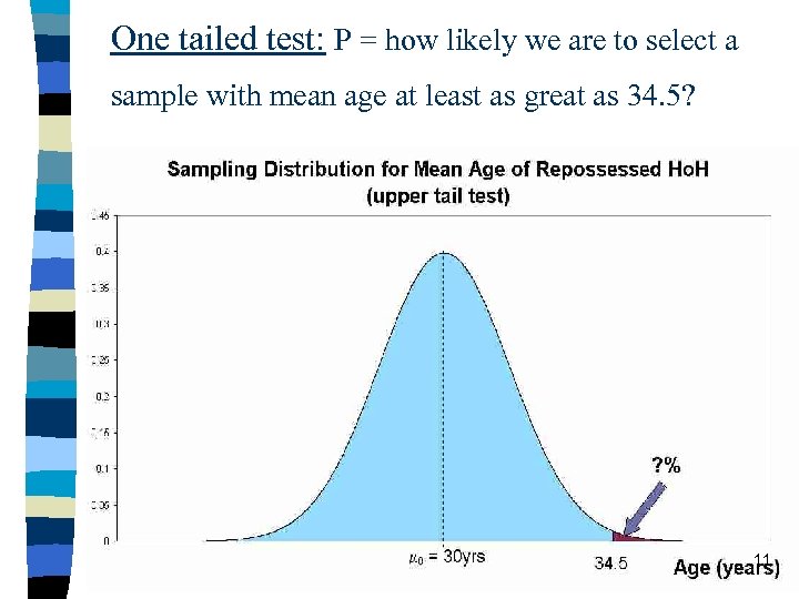
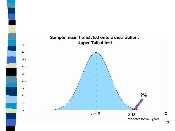
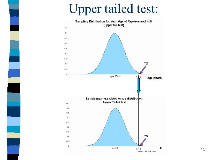
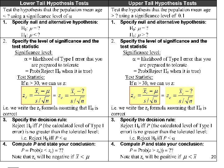
One tailed test: P = how likely we are to select a sample with mean age at least as great as 34. 5? 11

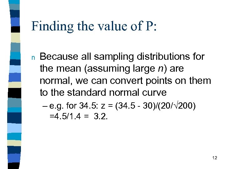
Finding the value of P: n Because all sampling distributions for the mean (assuming large n) are normal, we can convert points on them to the standard normal curve – e. g. for 34. 5: z = (34. 5 - 30)/(20/ 200) =4. 5/1. 4 = 3. 2. 12

13

14

Upper tailed test: 15

Two tailed test: 16

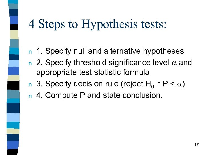
4 Steps to Hypothesis tests: n n 1. Specify null and alternative hypotheses 2. Specify threshold significance level a and appropriate test statistic formula 3. Specify decision rule (reject H 0 if P < a) 4. Compute P and state conclusion. 17

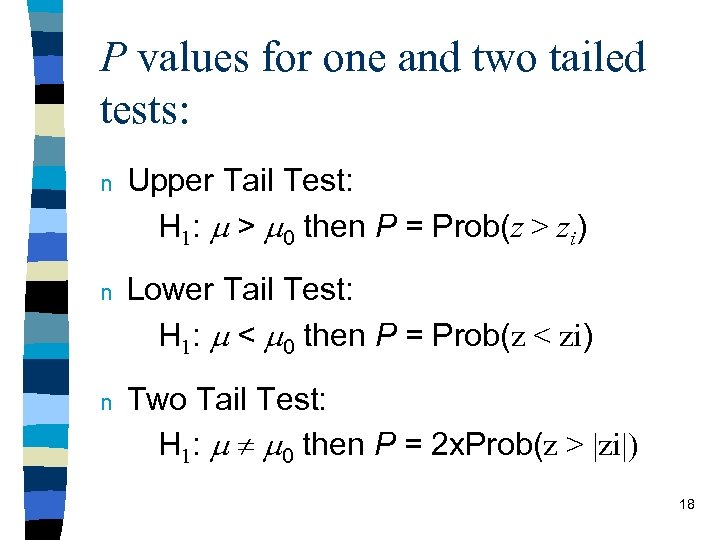
P values for one and two tailed tests: n Upper Tail Test: H 1: m > m 0 then P = Prob(z > zi) n Lower Tail Test: H 1: m < m 0 then P = Prob(z < zi) n Two Tail Test: H 1: m m 0 then P = 2 x. Prob(z > |zi|) 18

19

20

5. Overview of the Course: 21

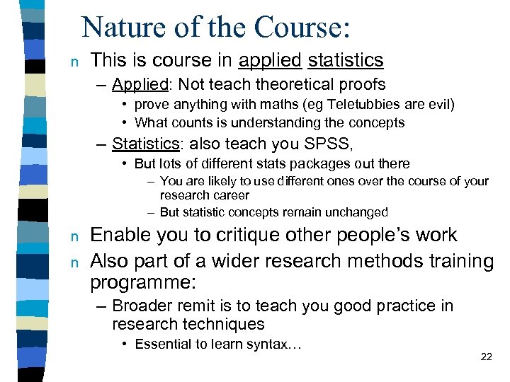
Nature of the Course: n This is course in applied statistics – Applied: Not teach theoretical proofs • prove anything with maths (eg Teletubbies are evil) • What counts is understanding the concepts – Statistics: also teach you SPSS, • But lots of different stats packages out there – You are likely to use different ones over the course of your research career – But statistic concepts remain unchanged n n Enable you to critique other people’s work Also part of a wider research methods training programme: – Broader remit is to teach you good practice in research techniques • Essential to learn syntax… 22

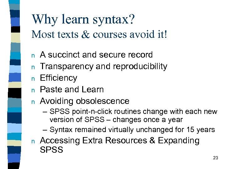
Why learn syntax? Most texts & courses avoid it! n n n A succinct and secure record Transparency and reproducibility Efficiency Paste and Learn Avoiding obsolescence – SPSS point-n-click routines change with each new version of SPSS – changes once a year – Syntax remained virtually unchanged for 15 years n Accessing Extra Resources & Expanding SPSS 23

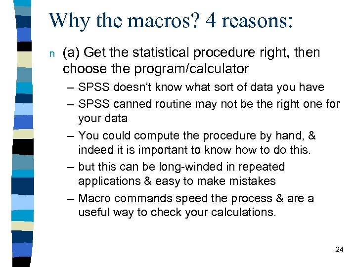
Why the macros? 4 reasons: n (a) Get the statistical procedure right, then choose the program/calculator – SPSS doesn’t know what sort of data you have – SPSS canned routine may not be the right one for your data – You could compute the procedure by hand, & indeed it is important to know how to do this. – but this can be long-winded in repeated applications & easy to make mistakes – Macro commands speed the process & are a useful way to check your calculations. 24

n (b) Critiquing/Analysing Published Work – SPSS routines can only be used if you have the original data – Not much use if you want to critique or analyse someone else’s published research • E. g. Newspaper examples in M&S tutorial • E. g. United Nations crime survey • E. g. MPPI paper by Pryce & Keoghan – If all you can do is the point-n-click stuff in SPSS you are going to be severely hampered in what you can do. – The Macro commands written specifically for the course only need summary info (n, xbar, sd, prop. ) • Publicly available via the downloads page of www. geebeejey. co. uk 25

n (c) Working with standard texts – The exercises and examples in standard statistical texts (such as Moore and Mc. Cabe) usually only provide summary information not the original data. – Can’t use SPSS to do these examples or to check your results 26

n (d) Encourages awareness & development of Macros – SPSS’s greatest strength: • Customisability/expandability – Actually don’t need to be good at statistics to use macros • You can use macros to do anything: – Manipulate data, – Automate repetitive tasks – Formalise and automate complex calculations – Writing SPSS macros is actually a good way to acquire basic programming skills – In real-life applied research, most of your time is taken up with non-statistical manipulation of data • Learning how to write your own macros or use other people’s will greatly increase your productivity & employability! 27

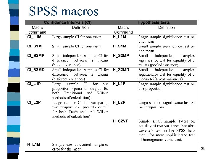
SPSS macros 28

Guide to Reading: n Essential reading (recommended for purchase): – Pryce, G. Inference and Statistics in SPSS • Lab exercises drawn from this book. n Usually recommended a book on statistics & a book on SPSS: – E. g. Moore & Mc. Cabe (£ 40) -- stats – E. g. Field (£ 25+) -- SPSS – M&M and Field = 2 great books but 4 major problems: 29

2 great books but 4 major problems: – 1. Cost (to buy both comes to approx £ 65) • many students have tried to make do without one or the other & struggled. – 2. Length • 600 pages (M&M) + 832 pages (Field) – 3. Content: neither geared to business & soc. sci. • Field: too shallow/applied: – Covers huge spectrum of topics (useful for Quants II) – does not cover some of the basic material we need to do » tends to cover what can be achieved in SPSS » Does not use macros » Does not teach syntax • M&M: too deep/theoretical – The Rolls Royce of introductory texts but does not teach SPSS – But would take 2 semesters to cover material in this depth & learn SPSS – 4. Integration • Leaves you the student with the task of combining the two 30

Advantages of Pryce I&S: – 1. Cost • Pryce = £ 22 + P&P (special price of £ 20 this week) – M&M + Field = £ 65 – 2. Length • Pryce = 200 pages + supplement with further reading – 600 pages (M&M) + 832 pages (Field) – 3. Content: • Pryce: – – – tries to strike the right balance between theory & application Based in SPSS Teaches syntax Uses the macros Geared to business and social science Based on worked examples & exercises – 4. Integration • Pryce tries to integrate learning inference with learning SPSS • But macros will also allow you do do the Moore & Mc. Cabe type of exercise should you want to get more practice 31

Disadvantages of Pryce I&S: n 1. First edition: – A few glitches here & there… – But, rare edition because only a small print run • • n valuable as a collectors item if you keep it for 20 years. Glitches add value – ask a stamp collector Even more valuable if I sign it. Makes a great Xmas gift for friends & family. 2. Wire comb binding – But actually better for working next to PC n 3. I’m biased in my recommendation! – But correct, of course. 32

Feedback forms… 33