Facilities Design S S Heragu Industrial Engineering Department

Facilities Design S. S. Heragu Industrial Engineering Department University of Louisville

Chapter 12: Advanced Location Models

Chapter 12: Advanced Location Models 12. 1 12. 2 12. 3 INTRODUCTION LOCATION MODELS 12. 2. 1 Multiple-Facility Problems with Rectilinear Distances 12. 2. 2 Multiple-Facility Problems with Euclidean Distances ALLOCATION MODELS 12. 3. 1 Network Flow Model 12. 3. 2 Two-Stage Transportation Model 12. 3. 3 Vehicle Routing Problem

Chapter 12: Advanced Location Models 12. 4 12. 5 LOCATION-ALLOCATION MODELS 12. 4. 1 Set Covering Model 12. 4. 2 Uncapacitated Location-Allocation Model 12. 4. 3 Comprehensive Location. Allocation Model SUMMARY

Introduction - How many new facilities are to be located in the distribution network consisting of previously established facilities and customers? Where should they be located? How large should each new facility be? In other words, what is the capacity of the new facility?

Introduction - How should customers be assigned to the new and existing facilities? More specifically, which facilities should be serving each customer? Can more than one facility serve a customer?

12. 2 LOCATION MODELS

12. 2. 1 Multiple-Facility Problems with Rectilinear Distances

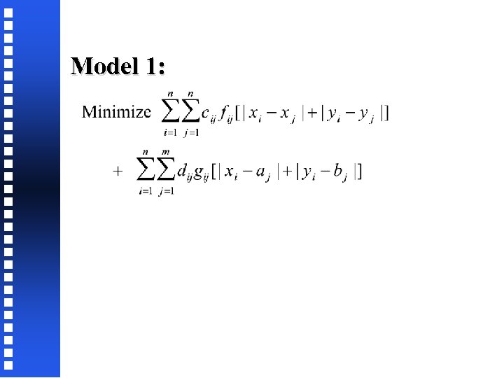Model 1:

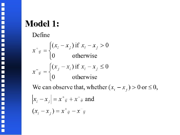Model 1:

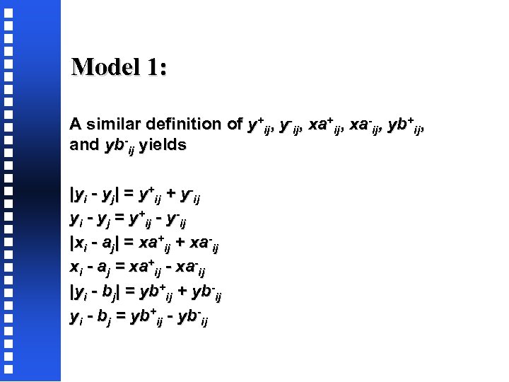Model 1: A similar definition of y+ij, y-ij, xa+ij, xa-ij, yb+ij, and yb-ij yields |yi - yj| = y+ij + y-ij yi - yj = y+ij - y-ij |xi - aj| = xa+ij + xa-ij xi - aj = xa+ij - xa-ij |yi - bj| = yb+ij + yb-ij yi - bj = yb+ij - yb-ij

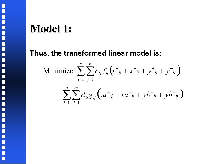Model 1: Thus, the transformed linear model is:

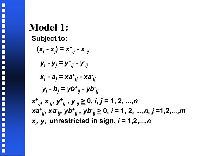Model 1: Subject to: (xi - xj) = x+ij - x-ij yi - yj = y+ij - y-ij xi - aj = xa+ij - xa-ij yi - bj = yb+ij - yb-ij x+ij, x-ij, y+ij , y-ij > 0, i, j = 1, 2, . . . , n xa+ij, xa-ij, yb+ij , yb-ij > 0, i = 1, 2, . . . , n, j =1, 2, . . . , m xi, yi unrestricted in sign, i = 1, 2, . . . , n

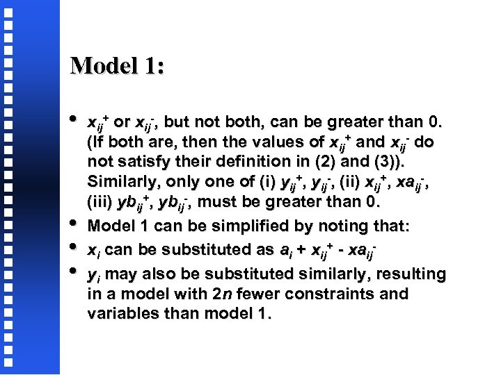Model 1: • • xij+ or xij-, but not both, can be greater than 0. (If both are, then the values of xij+ and xij- do not satisfy their definition in (2) and (3)). Similarly, only one of (i) yij+, yij-, (ii) xij+, xaij-, (iii) ybij+, ybij-, must be greater than 0. Model 1 can be simplified by noting that: xi can be substituted as ai + xij+ - xaijyi may also be substituted similarly, resulting in a model with 2 n fewer constraints and variables than model 1.

Example 1: • Tires and Brakes, Inc. , is an automobile service company specializing in tire and brake replacement. It has four service centers in a metropolitan area and a warehouse that supplies tires, brakes and other components to the service centers. The company manager has determined that he needs to add two more warehouses so as to improve component delivery service.

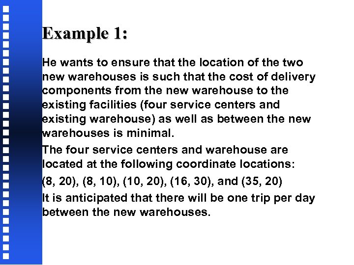Example 1: He wants to ensure that the location of the two new warehouses is such that the cost of delivery components from the new warehouse to the existing facilities (four service centers and existing warehouse) as well as between the new warehouses is minimal. The four service centers and warehouse are located at the following coordinate locations: (8, 20), (8, 10), (10, 20), (16, 30), and (35, 20) It is anticipated that there will be one trip per day between the new warehouses.

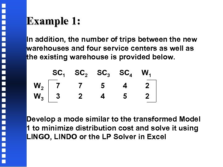Example 1: In addition, the number of trips between the new warehouses and four service centers as well as the existing warehouse is provided below. SC 1 W 2 W 3 SC 2 SC 3 SC 4 W 1 7 3 7 2 5 4 4 5 2 2 Develop a mode similar to the transformed Model 1 to minimize distribution cost and solve it using LINGO, LINDO or the LP Solver in Excel

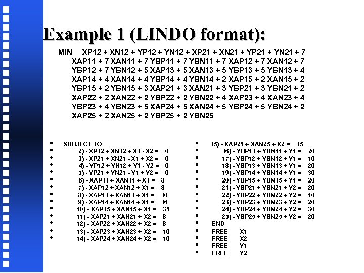Example 1 (LINDO format): MIN XP 12 + XN 12 + YP 12 + YN 12 + XP 21 + XN 21 + YP 21 + YN 21 + 7 XAP 11 + 7 XAN 11 + 7 YBP 11 + 7 YBN 11 + 7 XAP 12 + 7 XAN 12 + 7 YBP 12 + 7 YBN 12 + 5 XAP 13 + 5 XAN 13 + 5 YBP 13 + 5 YBN 13 + 4 XAP 14 + 4 XAN 14 + 4 YBP 14 + 4 YBN 14 + 2 XAP 15 + 2 XAN 15 + 2 YBP 15 + 2 YBN 15 + 3 XAP 21 + 3 XAN 21 + 3 YBP 21 + 3 YBN 21 + 2 XAP 22 + 2 XAN 22 + 2 YBP 22 + 2 YBN 22 + 4 XAP 23 + 4 XAN 23 + 4 YBP 23 + 4 YBN 23 + 5 XAP 24 + 5 XAN 24 + 5 YBP 24 + 5 YBN 24 + 2 XAP 25 + 2 XAN 25 + 2 YBP 25 + 2 YBN 25 • • • • SUBJECT TO 2) - XP 12 + XN 12 + X 1 - X 2 = 3) - XP 21 + XN 21 - X 1 + X 2 = 4) - YP 12 + YN 12 + Y 1 - Y 2 = 5) - YP 21 + YN 21 - Y 1 + Y 2 = 6) - XAP 11 + XAN 11 + X 1 = 7) - XAP 12 + XAN 12 + X 1 = 8) - XAP 13 + XAN 13 + X 1 = 9) - XAP 14 + XAN 14 + X 1 = 10) - XAP 15 + XAN 15 + X 1 = 11) - XAP 21 + XAN 21 + X 2 = 12) - XAP 22 + XAN 22 + X 2 = 13) - XAP 23 + XAN 23 + X 2 = 14) - XAP 24 + XAN 24 + X 2 = 0 0 8 8 10 16 35 8 8 10 16 • • • • 15) - XAP 25 + XAN 25 + X 2 = 35 16) - YBP 11 + YBN 11 + Y 1 = 17) - YBP 12 + YBN 12 + Y 1 = 18) - YBP 13 + YBN 13 + Y 1 = 19) - YBP 14 + YBN 14 + Y 1 = 20) - YBP 15 + YBN 15 + Y 1 = 21) - YBP 21 + YBN 21 + Y 2 = 22) - YBP 22 + YBN 22 + Y 2 = 23) - YBP 23 + YBN 23 + Y 2 = 24) - YBP 24 + YBN 24 + Y 2 = 25) - YBP 25 + YBN 25 + Y 2 = END FREE X 1 FREE X 2 FREE Y 1 FREE Y 2 20 10 20 30 20

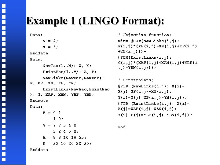Example 1 (LINGO Format): Data: N = 2; M = 5; Enddata Sets: New. Fac/1. . N/: X, Y; Exist. Fac/1. . M/: A, B; New. Links(New. Fac, New. Fac): F, XP, XN, YP, YN; Exist. Links(New. Fac, Exist. Fac ): G, XAP, XAN, YBP, YBN; Endsets Data: F = 0 1 1 0; G = 7 7 5 4 2 3 2 4 5 2; A = 8 8 10 16 35; B = 20 10 20 30 20; Enddata ! Objective function; Min= @SUM(New. Links(i, j): F(i, j)*(XP(i, j)+XN(i, j)+YP(i, j) +YN(i, j)))+ @SUM(Exist. Links(i, j): G(i, j)*(XAP(i, j)+XAN(i, j)+YBP(i , j)+YBN(i, j))); ! Constraints; @FOR (New. Links(i, j): X(i)X(j)=XP(i, j)-XN(i, j); Y(i)-Y(j)=YP(i, j)-YN(i, j)); @FOR (Exist. Links(i, j): X(i)A(j)=XAP(i, j)-XAN(i, j); Y(i)-B(j)=YBP(i, j)-YBN(i, j)); End

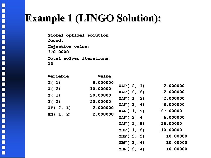Example 1 (LINGO Solution): Global optimal solution found. Objective value: 370. 0000 Total solver iterations: 16 Variable Value X( 1) 8. 000000 XAP( 2, 1) 2. 000000 X( 2) 10. 00000 XAP( 2, 2) 2. 000000 Y( 1) 20. 00000 XAN( 1, 3) 2. 000000 Y( 2) 20. 00000 XAN( 1, 4) 8. 000000 XP( 2, 1) 2. 000000 XAN( 1, 5) 27. 00000 XN( 1, 2) 2. 000000 XAN( 2, 4 6. 000000 XAN( 2, 5) 25. 00000 YBP( 1, 2) 10. 00000 YBP( 2, 2) 10. 00000 YBN( 1, 4) 10. 00000 YBN( 2, 4) 10. 00000

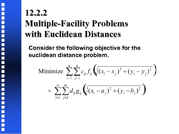12. 2. 2 Multiple-Facility Problems with Euclidean Distances Consider the following objective for the euclidean distance problem.

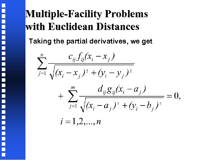Multiple-Facility Problems with Euclidean Distances Taking the partial derivatives, we get

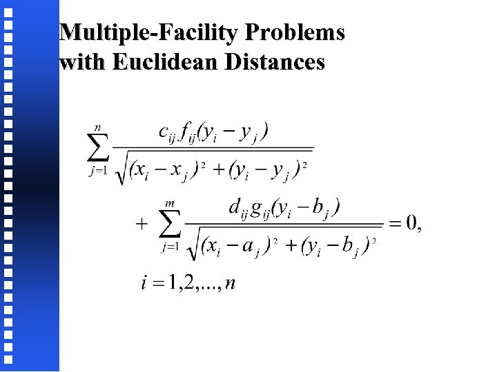Multiple-Facility Problems with Euclidean Distances

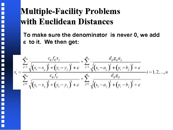Multiple-Facility Problems with Euclidean Distances To make sure the denominator is never 0, we add to it. We then get:

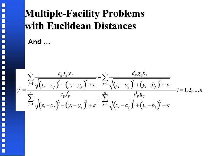Multiple-Facility Problems with Euclidean Distances And …

Example 2 Consider Example 1. Assuming the Euclidean metric is more appropriate and that Tire and Brakes, Inc. does not currently have a warehouse, determine where the two new warehouses are to be located.

12. 3 ALLOCATION MODEL

12. 3. 1 Network Flow Model

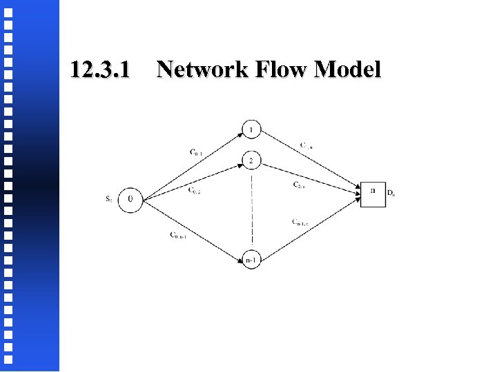
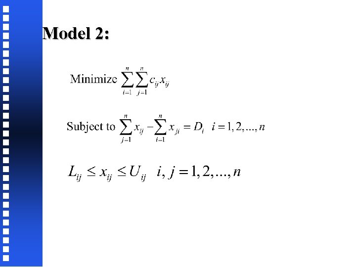
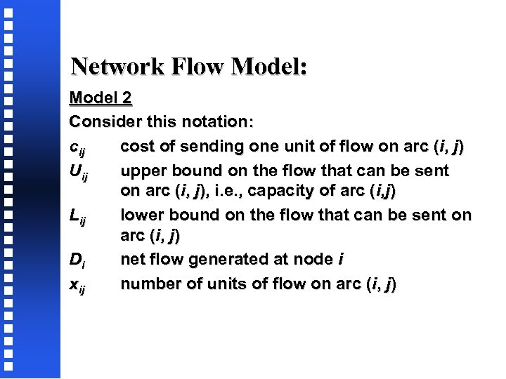Network Flow Model: Model 2 Consider this notation: cij cost of sending one unit of flow on arc (i, j) Uij upper bound on the flow that can be sent on arc (i, j), i. e. , capacity of arc (i, j) Lij lower bound on the flow that can be sent on arc (i, j) Di net flow generated at node i xij number of units of flow on arc (i, j)

Model 2:

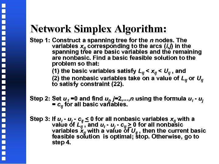Network Simplex Algorithm: Step 1: Construct a spanning tree for the n nodes. The variables xij corresponding to the arcs (i, j) in the spanning tree are basic variables and the remaining are nonbasic. Find a basic feasible solution to the problem so that: (1) the basic variables satisfy Lij < xij < Uij , and (2) the nonbasic variables take on a value of Lij or Uij to satisfy constraint (22). Step 2: Set u 1 =0 and find uj, j=2, . . . , n using the formula ui - uj = cij for all basic variables. Step 3: If ui - uj - cij < 0 for all nonbasic variables xij with a value of Lij , and ui - uj - cij > 0 for all nonbasic variables xij with a value of Uij , then the current basic feasible solution is optimal; stop. Otherwise, go to step 4.

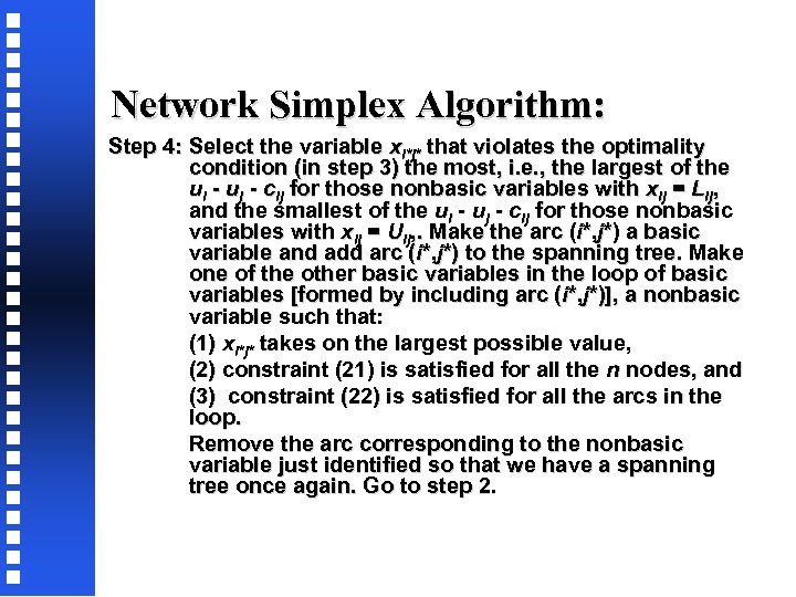Network Simplex Algorithm: Step 4: Select the variable xi*j* that violates the optimality condition (in step 3) the most, i. e. , the largest of the ui - uj - cij for those nonbasic variables with xij = Lij, and the smallest of the ui - uj - cij for those nonbasic variables with xij = Uij, . Make the arc (i*, j*) a basic variable and add arc (i*, j*) to the spanning tree. Make one of the other basic variables in the loop of basic variables [formed by including arc (i*, j*)], a nonbasic variable such that: (1) xi*j* takes on the largest possible value, (2) constraint (21) is satisfied for all the n nodes, and (3) constraint (22) is satisfied for all the arcs in the loop. Remove the arc corresponding to the nonbasic variable just identified so that we have a spanning tree once again. Go to step 2.

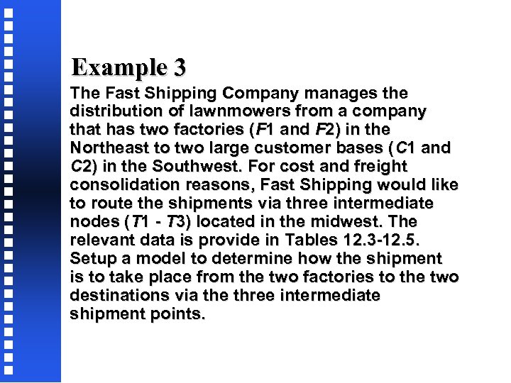Example 3 The Fast Shipping Company manages the distribution of lawnmowers from a company that has two factories (F 1 and F 2) in the Northeast to two large customer bases (C 1 and C 2) in the Southwest. For cost and freight consolidation reasons, Fast Shipping would like to route the shipments via three intermediate nodes (T 1 - T 3) located in the midwest. The relevant data is provide in Tables 12. 3 -12. 5. Setup a model to determine how the shipment is to take place from the two factories to the two destinations via the three intermediate shipment points.

Supply and Demand

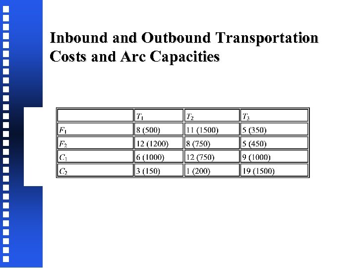Inbound and Outbound Transportation Costs and Arc Capacities

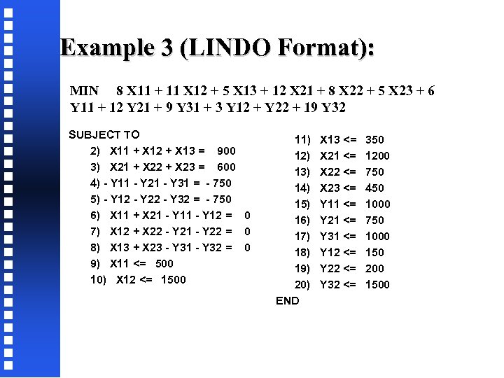Example 3 (LINDO Format): MIN 8 X 11 + 11 X 12 + 5 X 13 + 12 X 21 + 8 X 22 + 5 X 23 + 6 Y 11 + 12 Y 21 + 9 Y 31 + 3 Y 12 + Y 22 + 19 Y 32 SUBJECT TO 2) X 11 + X 12 + X 13 = 900 3) X 21 + X 22 + X 23 = 600 4) - Y 11 - Y 21 - Y 31 = - 750 5) - Y 12 - Y 22 - Y 32 = - 750 6) X 11 + X 21 - Y 12 = 0 7) X 12 + X 22 - Y 21 - Y 22 = 0 8) X 13 + X 23 - Y 31 - Y 32 = 0 9) X 11 <= 500 10) X 12 <= 1500 11) 12) 13) 14) 15) 16) 17) 18) 19) 20) END X 13 <= X 21 <= X 22 <= X 23 <= Y 11 <= Y 21 <= Y 31 <= Y 12 <= Y 22 <= Y 32 <= 350 1200 750 450 1000 750 1000 150 200 1500

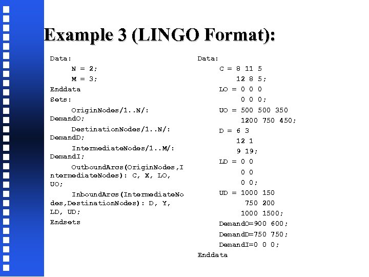Example 3 (LINGO Format): Data: N = 2; M = 3; Enddata Sets: Origin. Nodes/1. . N/: Demand. O; Destination. Nodes/1. . N/: Demand. D; Intermediate. Nodes/1. . M/: Demand. I; Outbound. Arcs(Origin. Nodes, I ntermediate. Nodes): C, X, LO, UO; Inbound. Arcs(Intermediate. No des, Destination. Nodes): D, Y, LD, UD; Endsets Data: C = 8 11 5 12 8 5; LO = 0 0 0 0; UO = 500 350 1200 750 450; D = 6 3 12 1 9 19; LD = 0 0; UD = 1000 150 750 200 1000 1500; Demand. O=900 600; Demand. D=750 750; Demand. I=0 0 0; Enddata

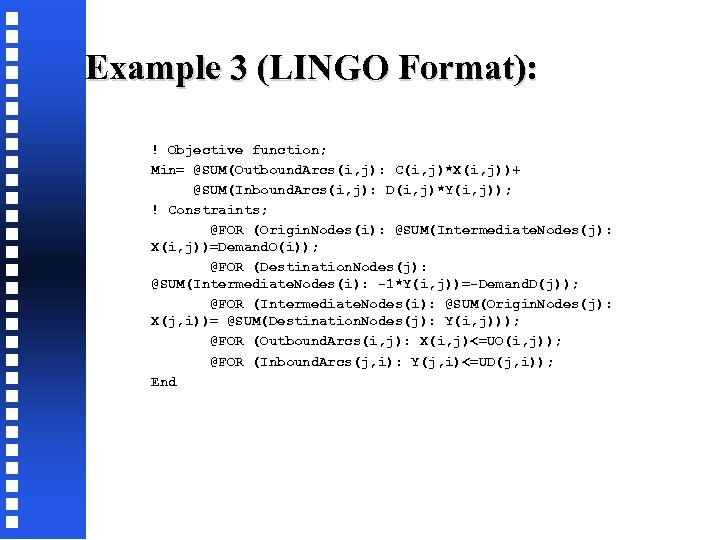Example 3 (LINGO Format): ! Objective function; Min= @SUM(Outbound. Arcs(i, j): C(i, j)*X(i, j))+ @SUM(Inbound. Arcs(i, j): D(i, j)*Y(i, j)); ! Constraints; @FOR (Origin. Nodes(i): @SUM(Intermediate. Nodes(j): X(i, j))=Demand. O(i)); @FOR (Destination. Nodes(j): @SUM(Intermediate. Nodes(i): -1*Y(i, j))=-Demand. D(j)); @FOR (Intermediate. Nodes(i): @SUM(Origin. Nodes(j): X(j, i))= @SUM(Destination. Nodes(j): Y(i, j))); @FOR (Outbound. Arcs(i, j): X(i, j)<=UO(i, j)); @FOR (Inbound. Arcs(j, i): Y(j, i)<=UD(j, i)); End

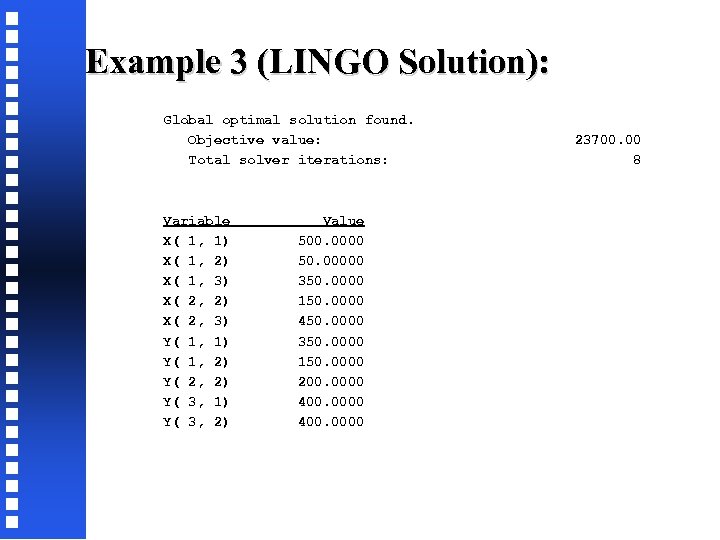Example 3 (LINGO Solution): Global optimal solution found. Objective value: 23700. 00 Total solver iterations: 8 Variable Value X( 1, 1) 500. 0000 X( 1, 2) 50. 00000 X( 1, 3) 350. 0000 X( 2, 2) 150. 0000 X( 2, 3) 450. 0000 Y( 1, 1) 350. 0000 Y( 1, 2) 150. 0000 Y( 2, 2) 200. 0000 Y( 3, 1) 400. 0000 Y( 3, 2) 400. 0000

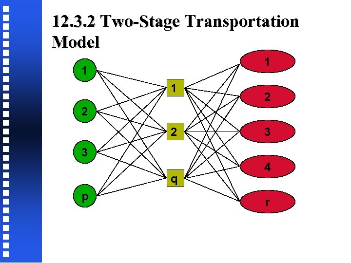12. 3. 2 Two-Stage Transportation Model 1 1 1 2 2 2 3 3 q p 4 r

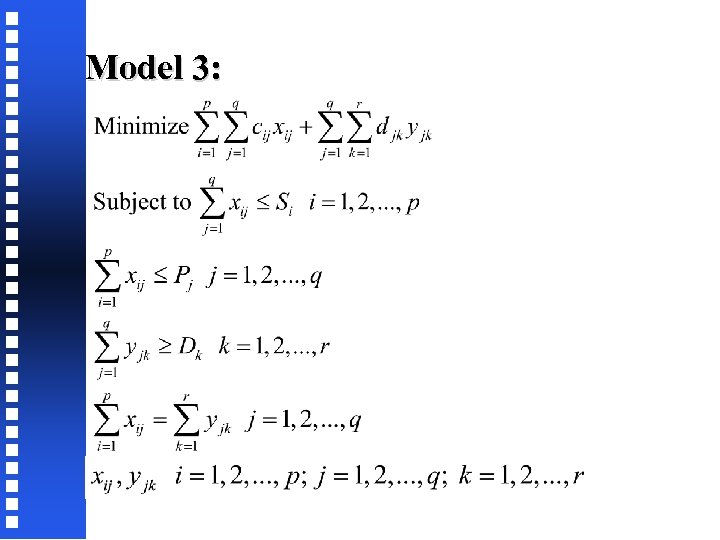
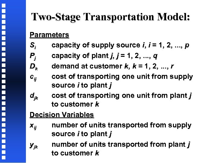Two-Stage Transportation Model: Parameters Si capacity of supply source i, i = 1, 2, . . . , p Pj capacity of plant j, j = 1, 2, . . . , q Dk demand at customer k, k = 1, 2, . . . , r cij cost of transporting one unit from supply source i to plant j djk cost of transporting one unit from plant j to customer k Decision Variables xij number of units transported from supply source i to plant j yjk number of units transported from plant j to customer k

Model 3:

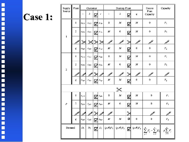
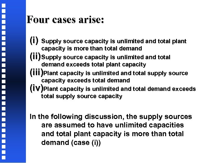Four cases arise: (i) Supply source capacity is unlimited and total plant capacity is more than total demand (ii) Supply source capacity is unlimited and total demand exceeds total plant capacity (iii)Plant capacity is unlimited and total supply source capacity exceeds total demand (iv)Plant capacity is unlimited and total demand exceeds total supply source capacity In the following discussion, the supply sources are assumed to have unlimited capacities and total plant capacity is more than total demand (case (i))

Case 1:

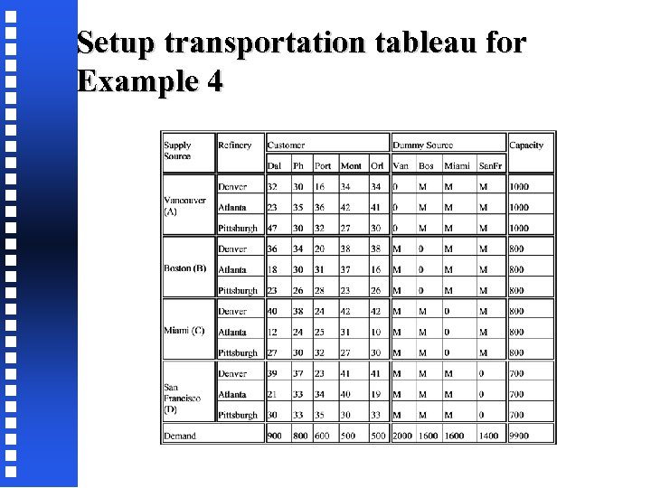
Example 4: 2 -Stage Distribution Problem: RIFIN Company has recently developed a new method of manufacturing a type of chemical. It involves refining a certain raw material which can be obtained from four overseas suppliers A, B, C, D who have access to the four ports at Vancouver, Boston, Miami, and San Francisco, respectively. RIFIN wants to determine the location of plants at which the chemical will be refined. The chemical, once refined, will be transported via trucks to five outlets located at Dallas, Phoenix, Portland, Montreal and Orlando.

Example 4: After an initial study, the choice of location for RIFIN’s refineries has narrowed down to Denver, Atlanta and Pittsburgh. Assume that one unit of raw material is required to make one unit of chemical. The amount of raw material from each potential refinery as well as the cost of trucking the chemical to outlets are also provided below. Determine the location of RIFIN’s refining plants, capacities at these plants and distribution pattern for the raw material and processed chemical.

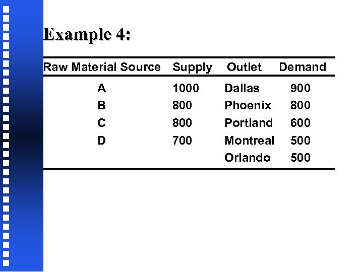Example 4: Raw Material Source Supply A B C D 1000 800 700 Outlet Dallas Phoenix Portland Montreal Orlando Demand 900 800 600 500

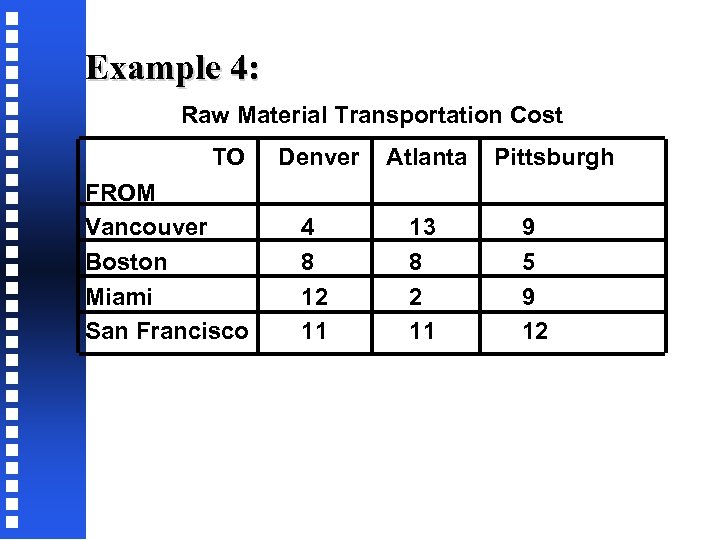Example 4: Raw Material Transportation Cost TO FROM Vancouver Boston Miami San Francisco Denver Atlanta 4 8 12 11 13 8 2 11 Pittsburgh 9 5 9 12

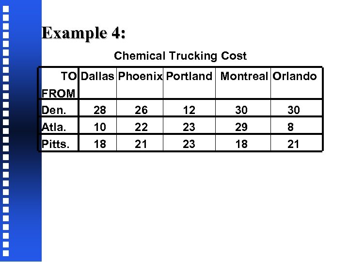Example 4: Chemical Trucking Cost TO Dallas Phoenix Portland Montreal Orlando FROM Den. 28 26 12 30 30 Atla. 10 22 23 29 8 Pitts. 18 21 23 18 21

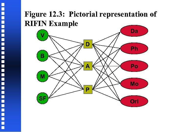Figure 12. 3: Pictorial representation of RIFIN Example Da V D Ph B A Po M P SF Mo Orl

Setup transportation tableau for Example 4

Solution: The transportation problem may be solved to yield the solution indicated in the following figure. Notice that the solution indicates that refineries be built at all locations.

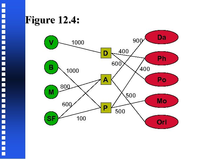Figure 12. 4: V 900 1000 D B M 600 Po A 800 500 P 100 Ph 400 1000 600 SF 400 Da Mo 500 Orl

12. 3. 3 Vehicle Routing Problem Determine the number of vehicles required to: (1)serve its customers (pick-up or deliver parcels) so that each customer is visited once and only once per day (2)the vehicle capacity is not exceeded, and (3)the total travel time is minimized

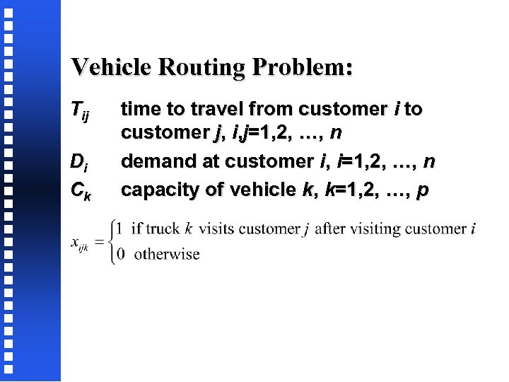Vehicle Routing Problem: Tij Di Ck time to travel from customer i to customer j, i, j=1, 2, …, n demand at customer i, i=1, 2, …, n capacity of vehicle k, k=1, 2, …, p

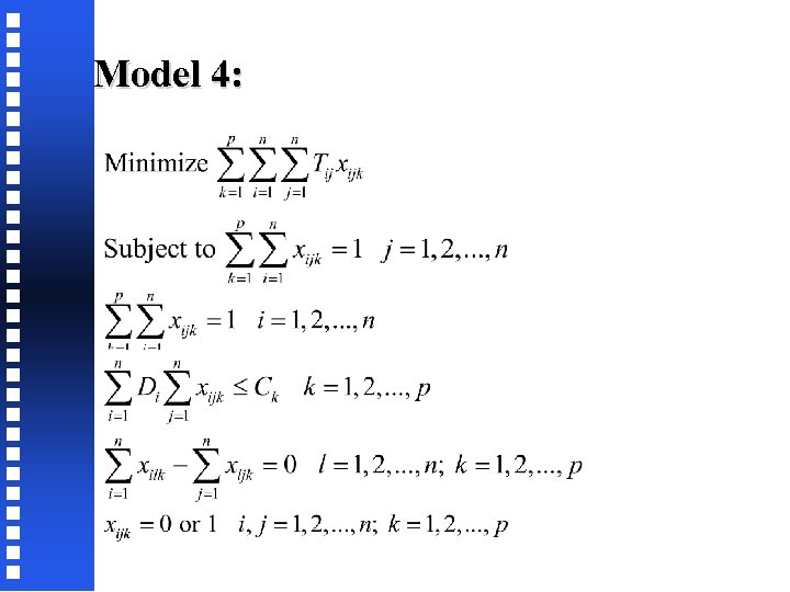Model 4:

12. 4 LOCATION-ALLOCATION MODELS

12. 4. 1 Set Covering Model

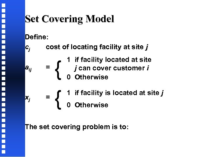Set Covering Model Define: cj cost of locating facility at site j aij xj = = { { 1 if facility located at site j can cover customer i 0 Otherwise 1 if facility is located at site j 0 Otherwise The set covering problem is to:

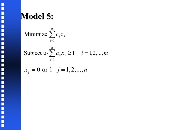Model 5:

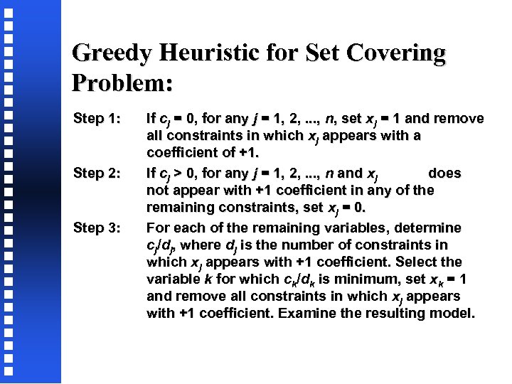Greedy Heuristic for Set Covering Problem: Step 1: Step 2: Step 3: If cj = 0, for any j = 1, 2, . . . , n, set xj = 1 and remove all constraints in which xj appears with a coefficient of +1. If cj > 0, for any j = 1, 2, . . . , n and xj does not appear with +1 coefficient in any of the remaining constraints, set xj = 0. For each of the remaining variables, determine cj/dj, where dj is the number of constraints in which xj appears with +1 coefficient. Select the variable k for which ck/dk is minimum, set xk = 1 and remove all constraints in which xj appears with +1 coefficient. Examine the resulting model.

Greedy Heuristic for Set Covering Problem: Step 4 If there are no more constraints, set all the remaining variables to 0 and stop. Otherwise go to step 1. We illustrate the above greedy heuristic with an example.

Example 5: A rural country administration wants to locate several medical emergency response units so that it can respond to calls within the county within eight minutes of the call. The county is divided into seven population zones. The distance between the centers of each pair of zones is known and is given in the matrix below.

Figure 12. 5: [dij] = 1 2 3 4 5 6 7 1 0 8 50 9 50 30 8 2 4 0 13 11 8 5 5 3 12 15 0 8 4 7 9 4 6 60 8 0 10 9 7 5 15 7 6 9 0 3 25 6 10 2 5 10 2 0 27 7 8 3 9 3 27 27 0

Example 5: The response units can be located in the center of population zones 1 through 7 at a cost (in hundreds of thousands of dollars) of 100, 80, 120 110, 90, and 110 respectively. Assuming the average travel speed during an emergency to be 60 miles per hour, formulate an appropriate set covering model to determine where the units are to be located and how the population zones are to be covered and solve the model using the greedy heuristic.

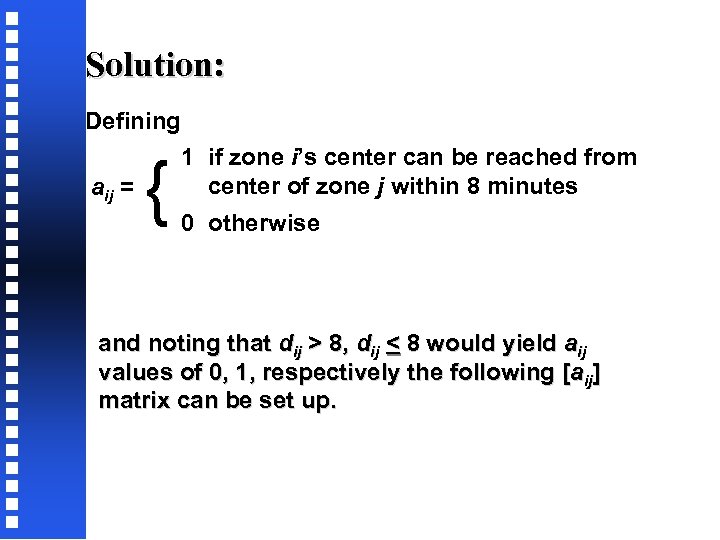Solution: Defining aij = { 1 if zone i’s center can be reached from center of zone j within 8 minutes 0 otherwise and noting that dij > 8, dij < 8 would yield aij values of 0, 1, respectively the following [aij] matrix can be set up.

Solution: [aij] = 1 2 3 4 5 6 7 1 1 1 0 0 1 2 1 1 0 0 1 1 1 3 0 0 1 1 0 4 1 0 1 1 0 0 1 5 0 1 1 0 6 0 1 1 0 The corresponding set covering model is: 7 1 1 0 0 1

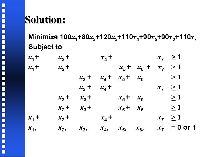Solution: Minimize 100 x 1+80 x 2+120 x 3+110 x 4+90 x 5+90 x 6+110 x 7 Subject to x 1 + x 2 + x 4 + x 7 > 1 x 1 + x 2 + x 5 + x 6 + x 7 > 1 x 3 + x 4 + x 5 + x 6 >1 x 3 + x 4 + x 7 > 1 x 2 + x 3 + x 5 + x 6 >1 x 1 + x 2 + x 4 + x 7 > 1 x 1, x 2, x 3, x 4, x 5, x 6, x 7 = 0 or 1

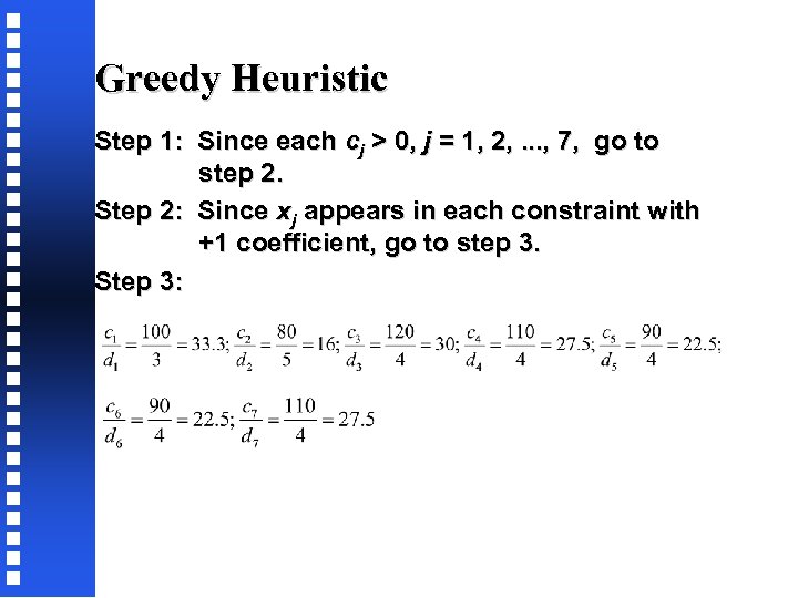Greedy Heuristic Step 1: Since each cj > 0, j = 1, 2, . . . , 7, go to step 2. Step 2: Since xj appears in each constraint with +1 coefficient, go to step 3. Step 3:

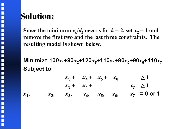Solution: Since the minimum ck/dk occurs for k = 2, set x 2 = 1 and remove the first two and the last three constraints. The resulting model is shown below. Minimize 100 x 1+80 x 2+120 x 3+110 x 4+90 x 5+90 x 6+110 x 7 Subject to x 3 + x 4 + x 5 + x 6 >1 x 3 + x 4 + x 7 > 1 x 1, x 2, x 3, x 4, x 5, x 6, x 7 = 0 or 1

Greedy Heuristic: Step 4: Since we have two constraints go to step 1. Step 1: Since c 1 > 0, j = 1, 3, 4, . . . , 7, go to step 2 Step 2: Since c 1 > 0 and x 1 does not appear in any of the constraints with +1 coefficient, set x 1 = 0.

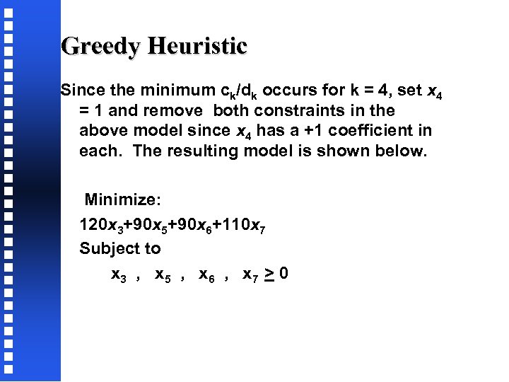Greedy Heuristic Since the minimum ck/dk occurs for k = 4, set x 4 = 1 and remove both constraints in the above model since x 4 has a +1 coefficient in each. The resulting model is shown below. Minimize: 120 x 3+90 x 5+90 x 6+110 x 7 Subject to x 3 , x 5 , x 6 , x 7 > 0

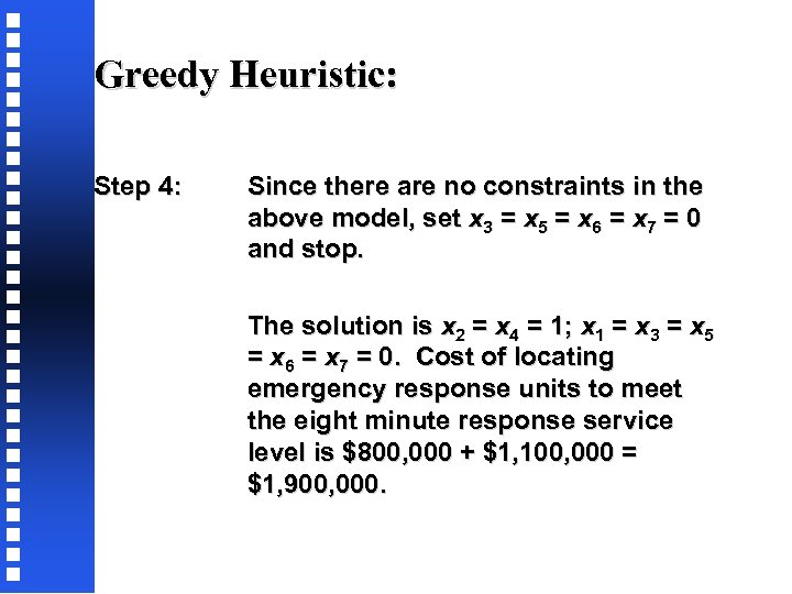Greedy Heuristic: Step 4: Since there are no constraints in the above model, set x 3 = x 5 = x 6 = x 7 = 0 and stop. The solution is x 2 = x 4 = 1; x 1 = x 3 = x 5 = x 6 = x 7 = 0. Cost of locating emergency response units to meet the eight minute response service level is $800, 000 + $1, 100, 000 = $1, 900, 000.

12. 4. 2 Uncapacitated Location-Allocation Model

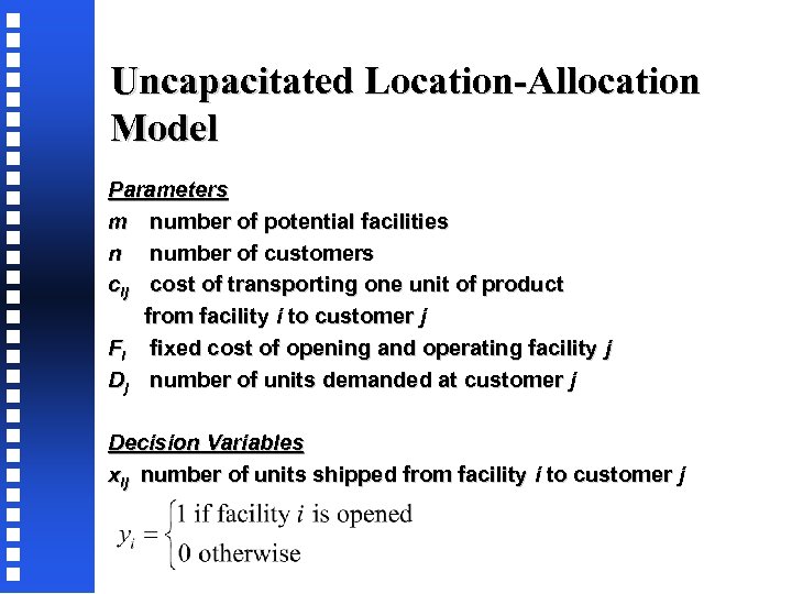Uncapacitated Location-Allocation Model Parameters m number of potential facilities n number of customers cij cost of transporting one unit of product from facility i to customer j Fi fixed cost of opening and operating facility j Dj number of units demanded at customer j Decision Variables xij number of units shipped from facility i to customer j

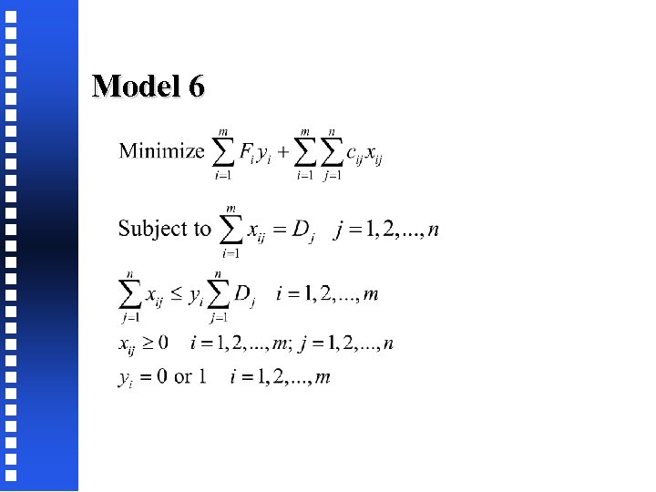Model 6

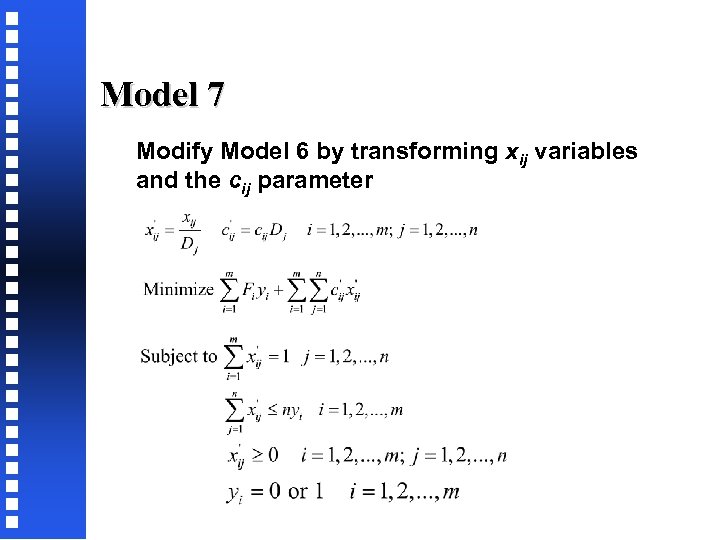Model 7 Modify Model 6 by transforming xij variables and the cij parameter

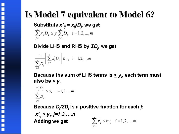Is Model 7 equivalent to Model 6? Substitute x’ij = xij/Dj, we get Divide LHS and RHS by ΣDj, we get Because the sum of LHS terms is < yi, each term must also be < yi Because Dj/ΣDj is a positive fraction for each j: x’ij < yi, j=1, 2, …, n Adding we get

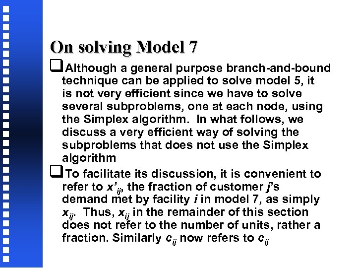On solving Model 7 q. Although a general purpose branch-and-bound technique can be applied to solve model 5, it is not very efficient since we have to solve several subproblems, one at each node, using the Simplex algorithm. In what follows, we discuss a very efficient way of solving the subproblems that does not use the Simplex algorithm q. To facilitate its discussion, it is convenient to refer to x’ij, the fraction of customer j’s demand met by facility i in model 7, as simply xij. Thus, xij in the remainder of this section does not refer to the number of units, rather a fraction. Similarly cij now refers to cij

On solving Model 7 q. The central idea of the branch-and-bound algorithm is based on the following result q. Suppose, at some stage of the branch-and-bound solution process, we are at a node where some facilities are closed (corresponding yi = 0), and some are open (yi = 1) and the remaining are free, i. e. , a decision whether to open or close has not yet been taken (0< yi <1). Let us define: q. S 0 as the set of facilities whose yi value is equal to 0; {i: yi = 0} q. S 1 as the set of facilities whose yi value is equal to 1; {i: yi = 1) q. S 2 as the set of facilities whose yi value is greater than 0 but less than 1; {i: 0 < yi < 1}

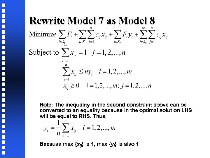Rewrite Model 7 as Model 8 Note: The inequality in the second constraint above can be converted to an equality because in the optimal solution LHS will be equal to RHS. Thus, Because max {xij} is 1, max {yi} is also 1

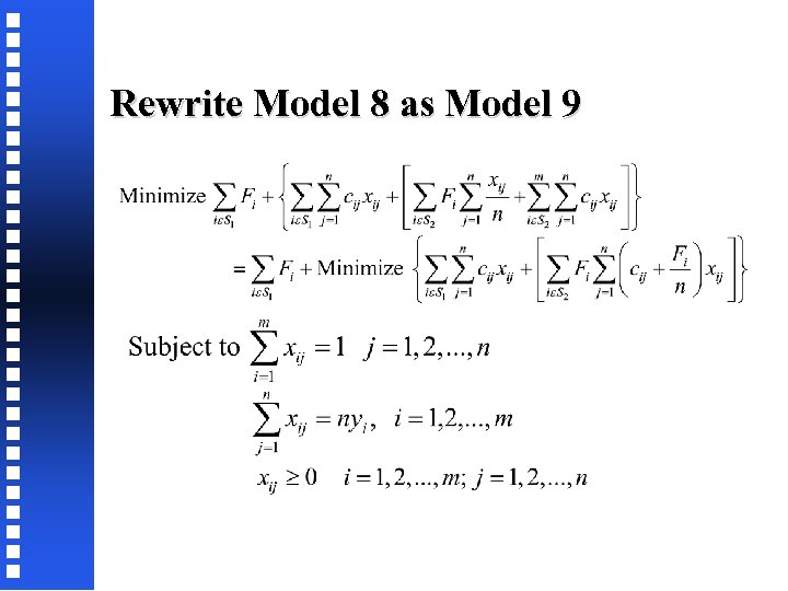Rewrite Model 8 as Model 9

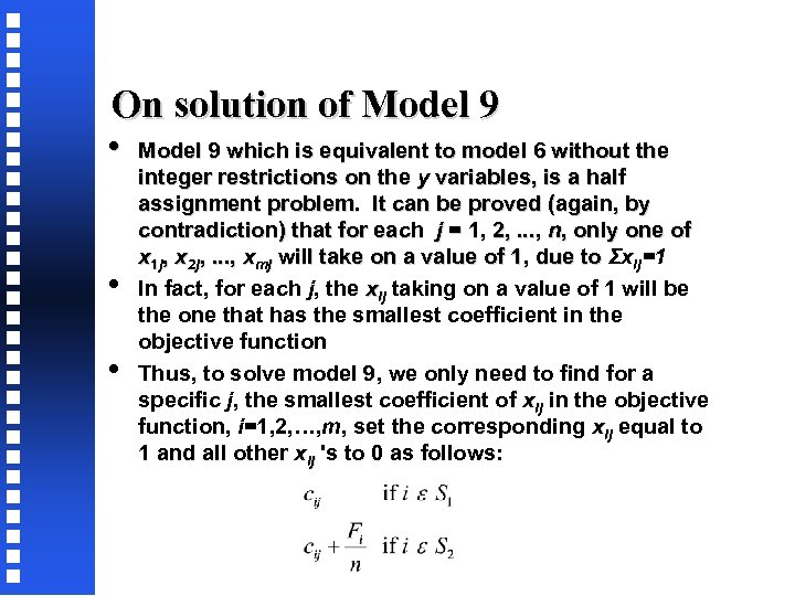On solution of Model 9 • • • Model 9 which is equivalent to model 6 without the integer restrictions on the y variables, is a half assignment problem. It can be proved (again, by contradiction) that for each j = 1, 2, . . . , n, only one of x 1 j, x 2 j, . . . , xmj will take on a value of 1, due to Σxij=1 In fact, for each j, the xij taking on a value of 1 will be the one that has the smallest coefficient in the objective function Thus, to solve model 9, we only need to find for a specific j, the smallest coefficient of xij in the objective function, i=1, 2, …, m, set the corresponding xij equal to 1 and all other xij 's to 0 as follows:

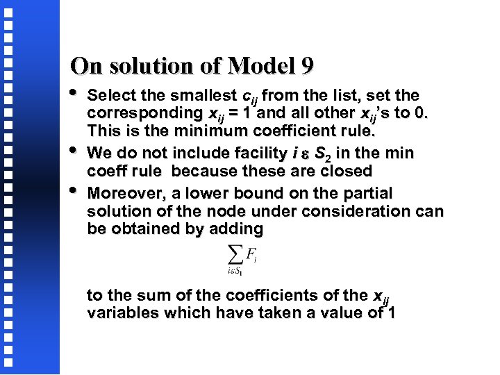On solution of Model 9 • Select the smallest cij from the list, set the • • corresponding xij = 1 and all other xij’s to 0. This is the minimum coefficient rule. We do not include facility i S 2 in the min coeff rule because these are closed Moreover, a lower bound on the partial solution of the node under consideration can be obtained by adding to the sum of the coefficients of the xij variables which have taken a value of 1

Branch-and-Bound Algorithm for Basic Location-Allocation Model

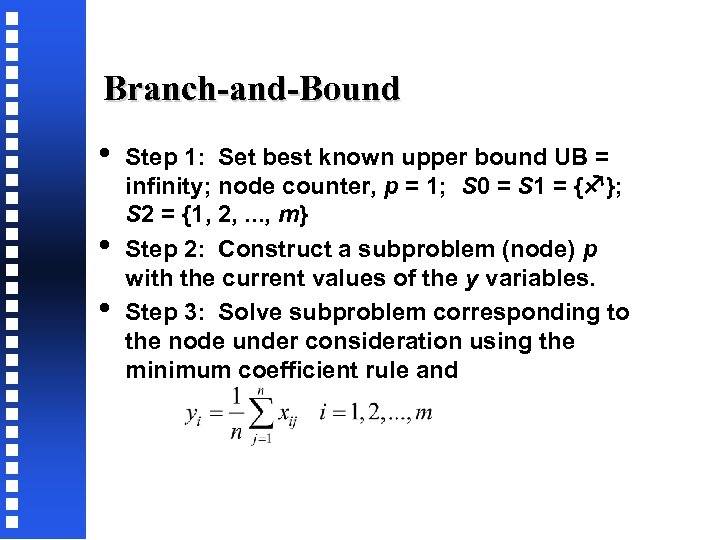Branch-and-Bound • • • Step 1: Set best known upper bound UB = infinity; node counter, p = 1; S 0 = S 1 = { }; S 2 = {1, 2, . . . , m} Step 2: Construct a subproblem (node) p with the current values of the y variables. Step 3: Solve subproblem corresponding to the node under consideration using the minimum coefficient rule and

Branch-and-Bound Step 4: If the solution is such that all y variables take on integer (0 or 1) values, go to step 7. Otherwise go to step 5. Step 5: Determine the lower bound of node p using model 7. Arbitrarily select one of the facilities, say k, which has taken on a fractional value for yk, i. e. , 0 < yk < 1 and create two subproblems (nodes) p+1 and p+2 as follows.

Branch-and-Bound Subproblem p+1 • Include facility k and others with a yk value of 0 in So; facilities with yk value of 1 in S 1; all other facilities in S 2 Subproblem p+2 • Include facility k and others with a yk value of 1 in S 1; facilities with yk value of 0 in S 0; all other facilities in S 2. If xkj = 1 for j = 1, 2, . . . , n, in the solution to subproblem p, remove each such customer j from consideration in subproblem p+2, and reduce n by the number of j’s for which xkj = 1

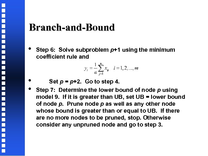Branch-and-Bound • Step 6: Solve subproblem p+1 using the minimum coefficient rule and • • Set p = p+2. Go to step 4. Step 7: Determine the lower bound of node p using model 9. If it is greater than UB, set UB = lower bound of node p. Prune node p as well as any other node whose bound is greater than or equal to UB. If there are no more nodes to be pruned, stop. Otherwise consider any unpruned node and go to step 3.

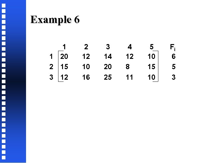
Example 6 The nation’s leading retailer Sam-Mart wants to establish its presence in the Northeast by opening five department stores. In order to serve the stores (whose locations have already been determined), the retailer wants to have a maximum of three distribution warehouses. The potential locations for these warehouses have already been selected and there are no practical limits on the size of the warehouses. The fixed cost (in hundreds of thousands of dollars) of building and operating the warehouse at each location is 6, 5, and 3, respectively.

Example 6 The variable cost of serving each warehouse from each of the potential warehouse locations is given below (again in hundreds of thousands of dollars). Determine how many warehouses are to be built and in what locations. Also determine how the customers (departmental stores) are to be served.

Example 6 1 1 20 2 15 3 12 2 12 10 16 3 14 20 25 4 12 8 11 5 10 15 10 Fi 6 5 3

Solution: Step 1: Set UB = infinity; node counter p = 1; S 0 = S 1 = { }; S 2 = {1, 2, 3}. Step 2: Minimum coefficient rule: Determine the xij coefficients as follows.

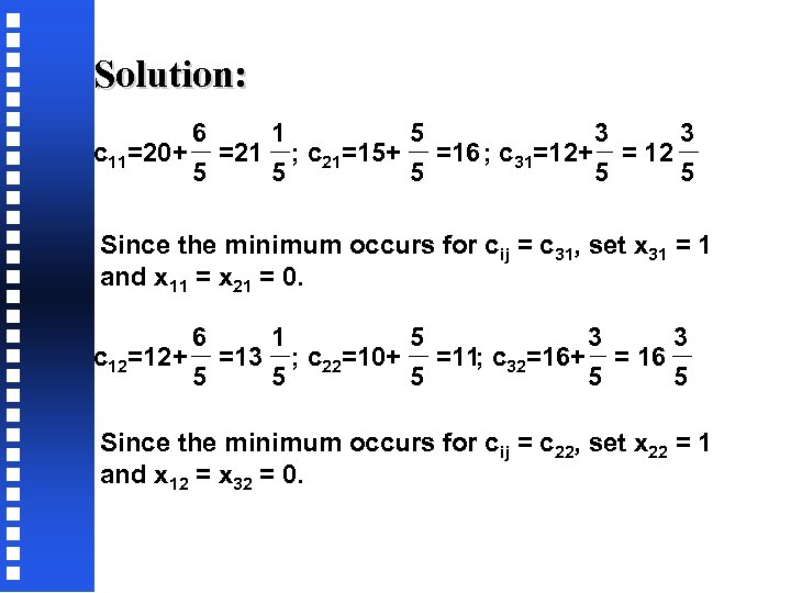Solution: 6 1 5 3 3 c 11=20+ =21 ; c 21=15+ =16 ; c 31=12+ = 12 5 5 5 Since the minimum occurs for cij = c 31, set x 31 = 1 and x 11 = x 21 = 0. 6 1 5 3 3 c 12=12+ =13 ; c 22=10+ =11; c 32=16+ = 16 5 5 5 Since the minimum occurs for cij = c 22, set x 22 = 1 and x 12 = x 32 = 0.

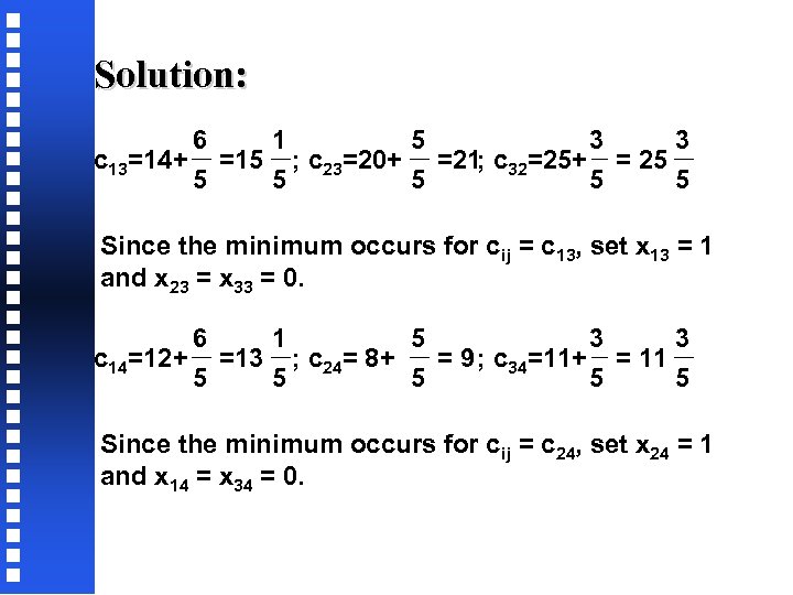Solution: 6 1 5 3 3 c 13=14+ =15 ; c 23=20+ =21; c 32=25+ = 25 5 5 Since the minimum occurs for cij = c 13, set x 13 = 1 and x 23 = x 33 = 0. 6 1 5 3 3 c 14=12+ =13 ; c 24= 8+ = 9 ; c 34=11+ = 11 5 5 5 Since the minimum occurs for cij = c 24, set x 24 = 1 and x 14 = x 34 = 0.

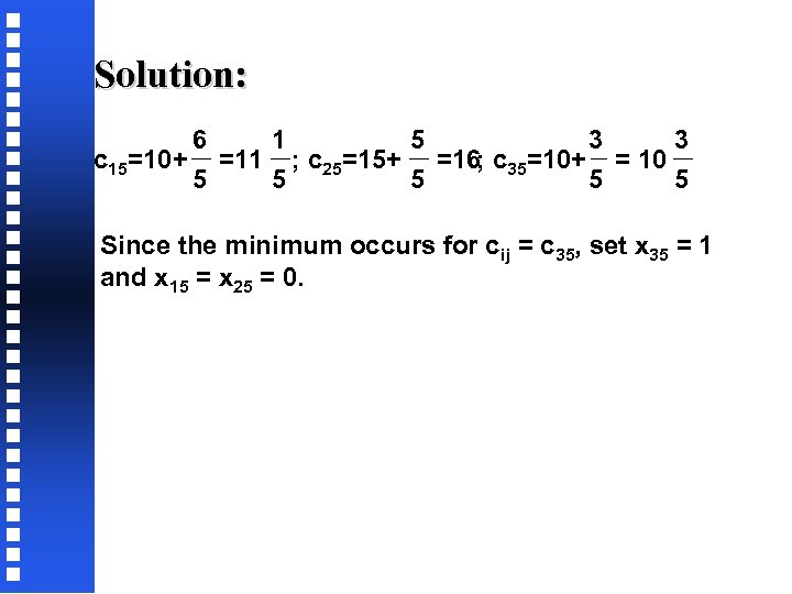Solution: 6 1 5 3 3 c 15=10+ =11 ; c 25=15+ =16; c 35=10+ = 10 5 5 5 Since the minimum occurs for cij = c 35, set x 35 = 1 and x 15 = x 25 = 0.

Solution: 1 1 1 y 1= [x 11+x 12+x 13+x 14+x 15]= [0+0+1+0+0]= 5 5 5 1 1 2 y 2= [x 21+x 22+x 23+x 24+x 25]= [0+1+0]= 5 5 5 1 1 2 y 3= [x 31+x 32+x 33+x 34+x 35]= [1+0+0+0+1]= 5 5 5

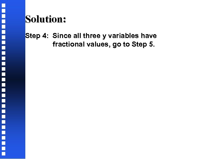Solution: Step 4: Since all three y variables have fractional values, go to Step 5.

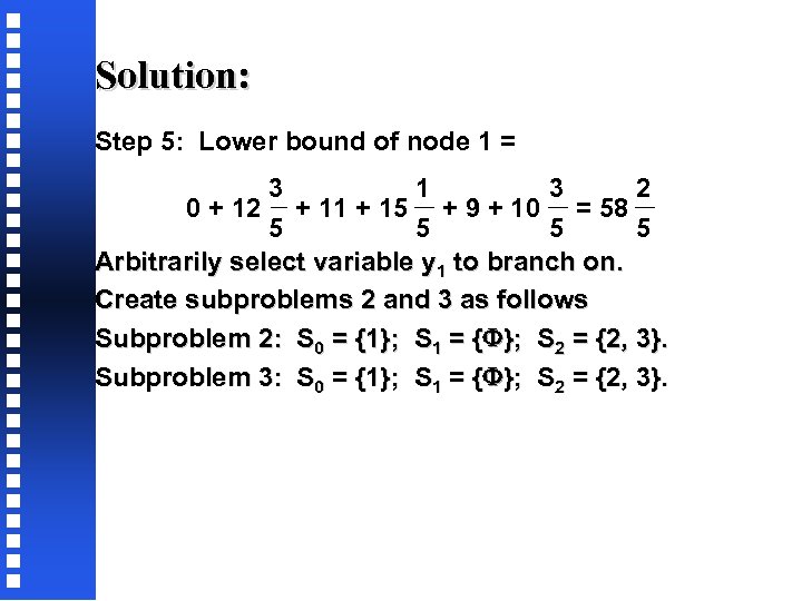Solution: Step 5: Lower bound of node 1 = 3 1 3 2 0 + 12 + 11 + 15 + 9 + 10 = 58 5 5 Arbitrarily select variable y 1 to branch on. Create subproblems 2 and 3 as follows Subproblem 2: S 0 = {1}; S 1 = { }; S 2 = {2, 3}. Subproblem 3: S 0 = {1}; S 1 = { }; S 2 = {2, 3}.

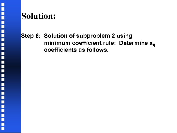Solution: Step 6: Solution of subproblem 2 using minimum coefficient rule: Determine xij coefficients as follows.

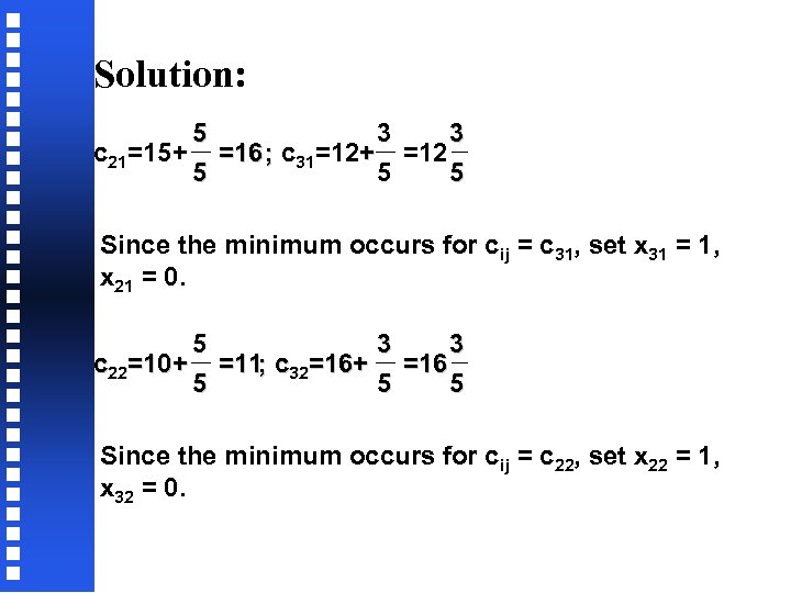Solution: 5 3 3 c 21=15+ =16 ; c 31=12+ =12 5 5 5 Since the minimum occurs for cij = c 31, set x 31 = 1, x 21 = 0. 5 3 3 c 22=10+ =11; c 32=16+ =16 5 5 5 Since the minimum occurs for cij = c 22, set x 22 = 1, x 32 = 0.

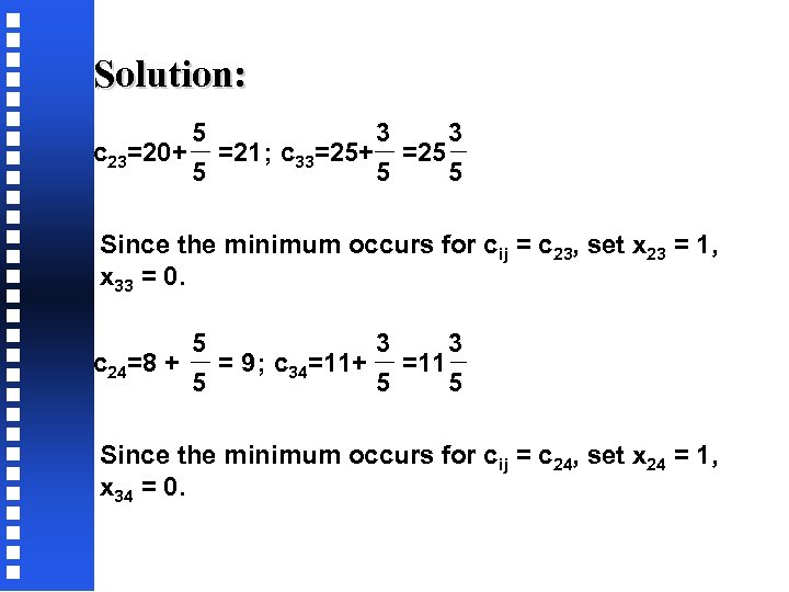Solution: 5 3 3 c 23=20+ =21 ; c 33=25+ =25 5 Since the minimum occurs for cij = c 23, set x 23 = 1, x 33 = 0. 5 3 3 c 24=8 + = 9 ; c 34=11+ =11 5 5 5 Since the minimum occurs for cij = c 24, set x 24 = 1, x 34 = 0.

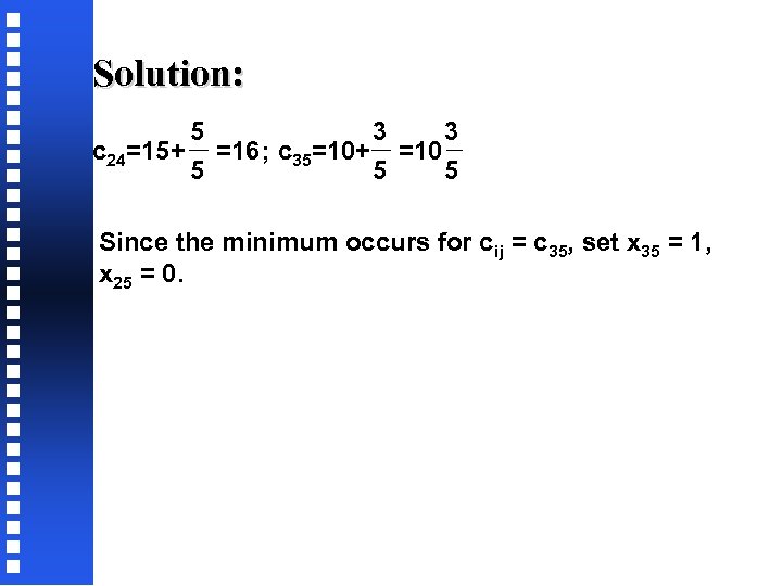Solution: 5 3 3 c 24=15+ =16 ; c 35=10+ =10 5 5 5 Since the minimum occurs for cij = c 35, set x 35 = 1, x 25 = 0.

Solution: 1 1 3 y 2= [x 21+x 22+x 23+x 24+x 25]= [0+1+1+1+0]= 5 5 5 1 1 2 y 3= [x 31+x 32+x 33+x 34+x 35]= [1+0+0+0+1]= 5 5 5

Solution: Solution of subproblem 3 using minimum coefficient rule: Determine xij coefficients as follows: Since x 13 = 1 in the solution to subproblem 1, remove store 1 from consideration in node 3 and other nodes emanting from node 3. Reduce n by 1, n=5 -1=4.

Solution: 5 1 3 3 c 11=20; c 21 =15+ =16 ; c 31=12+ =12 4 4 Since the minimum occurs for cij = c 31, set x 31 = 1 and x 11 = x 21 = 0. 5 1 3 3 c 12=12; c 22 =10+ =11 ; c 32=16+ =16 4 4 Since the minimum occurs for cij = c 22, set x 22 = 1 and x 12 = x 32 = 0.

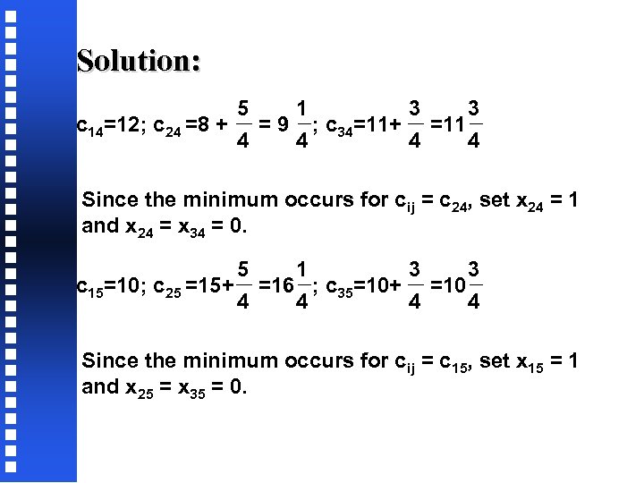Solution: 5 1 3 3 c 14=12; c 24 =8 + = 9 ; c 34=11+ =11 4 4 Since the minimum occurs for cij = c 24, set x 24 = 1 and x 24 = x 34 = 0. 5 1 3 3 c 15=10; c 25 =15+ =16 ; c 35=10+ =10 4 4 Since the minimum occurs for cij = c 15, set x 15 = 1 and x 25 = x 35 = 0.

Solution: 1 1 2 1 y 2= [x 21+x 22+x 24+x 25]= [0+1+1+0]= = 4 4 4 2 1 1 1 y 2= [x 31+x 32+x 34+x 35]= [1+0+0+0]= 4 4 4 Set p=1+2=3

Solution: Step 4: Since the solution for subproblem 2 is not all integer, go to step 5. We repeat steps 3, 4, 5, 6, and 7 until all the nodes are pruned. We then have an optimal solution. These steps are summarized in Table 2.

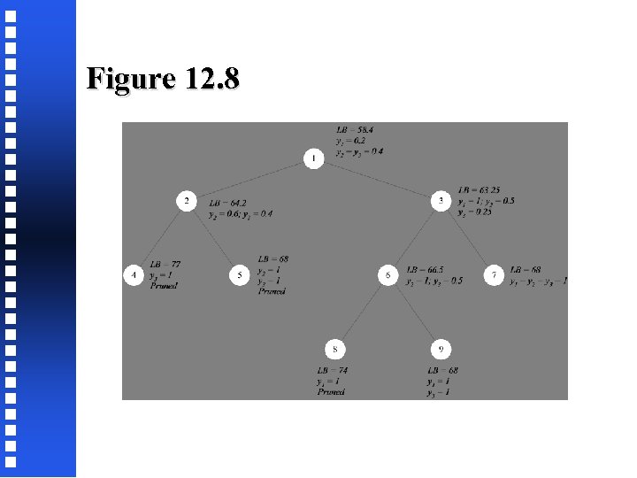Figure 12. 8

12. 5. 3 Comprehensive Location. Allocation Model

Comprehensive Location-Allocation Model Parameters Sij production capacity of product i at plant j Dil demand for product i at customer zone l Fk fixed cost of operating warehouse k Vik unit variable cost of handling product i at warehouse k Cijkl average unit cost of producing and transporting product i from plant j via warehouse k to customer l UCk Upper bound on the capacity of warehouse k LCk Lower bound on the capacity of warehouse k

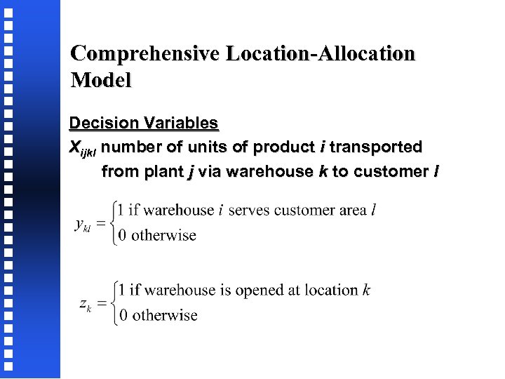Comprehensive Location-Allocation Model Decision Variables Xijkl number of units of product i transported from plant j via warehouse k to customer l

Model 10

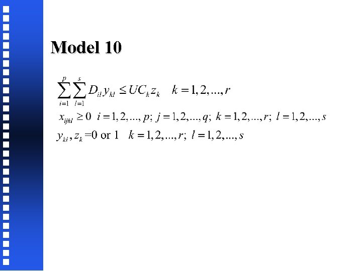Model 10

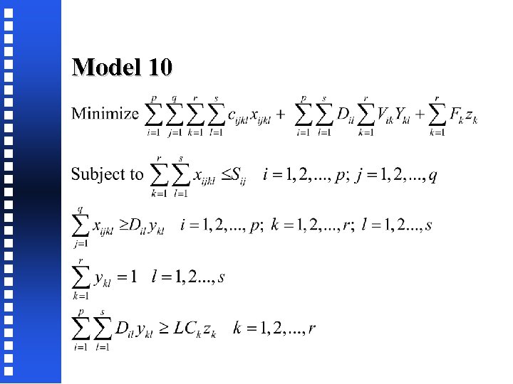
Comprehensive Location-Allocation Model We can easily add more linear constraints not involving xijkl variables to model 10 to: • Impose upper and lower limit on the number of warehouses that can be opened; • Enforce precedence relations among warehouses (e. g. , open warehouse at location 1 only if another is opened at location 3) • Enforce service constraints (e. g. , if it is decided to open a certain warehouse, then a specific customer area must be served by it) • Other constraints that can be added are discussed further in Geoffrion and Graves (1974). • Many of these constraints reduce the solution space, so they allow quicker solution of the model while giving the modeler much flexibility

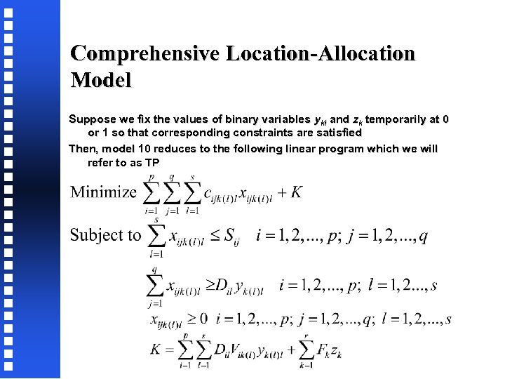Comprehensive Location-Allocation Model Suppose we fix the values of binary variables ykl and zk temporarily at 0 or 1 so that corresponding constraints are satisfied Then, model 10 reduces to the following linear program which we will refer to as TP

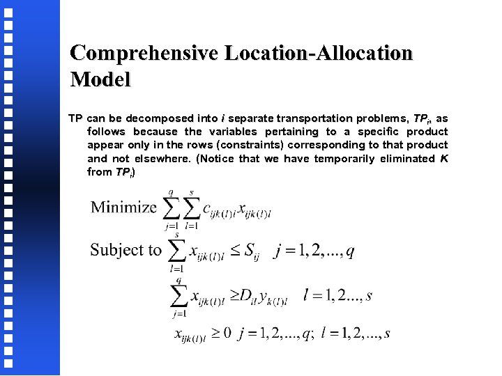Comprehensive Location-Allocation Model TP can be decomposed into i separate transportation problems, TPi, as follows because the variables pertaining to a specific product appear only in the rows (constraints) corresponding to that product and not elsewhere. (Notice that we have temporarily eliminated K from TPi)

Comprehensive Location-Allocation Model TP can be decomposed into i separate transportation problems, TPi, as follows because the variables pertaining to a specific product appear only in the rows (constraints) corresponding to that product and not elsewhere. (Notice that we have temporarily eliminated K from TPi)

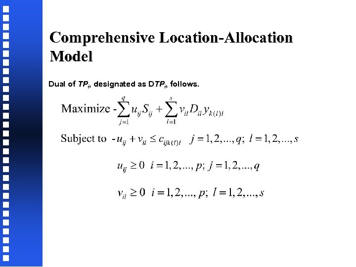Comprehensive Location-Allocation Model Dual of TPi, designated as DTPi, follows.

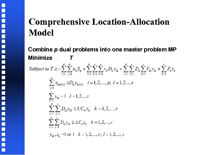Comprehensive Location-Allocation Model Combine p dual problems into one master problem MP Minimize T

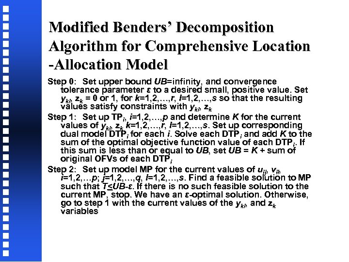Modified Benders’ Decomposition Algorithm for Comprehensive Location -Allocation Model Step 0: Set upper bound UB=infinity, and convergence tolerance parameter ε to a desired small, positive value. Set ykl, zk = 0 or 1, for k=1, 2, …, r, l=1, 2, …, s so that the resulting values satisfy constraints with ykl, zk Step 1: Set up TPi, i=1, 2, …, p and determine K for the current values of ykl, zk k=1, 2, …, r, l=1, 2, …, s. Set up corresponding dual model DTPi for each i. Solve each DTPi and add K to the sum of the optimal objective function value of each DTPi. If this sum is less than or equal to UB, set UB = K + sum of original OFVs of each DTPi Step 2: Set up model MP for the current values of uij, vil, i=1, 2, …p; j=1, 2, …, q, l=1, 2, …, s. Find a feasible solution to MP such that T

Example 7 The nation’s leading grocer, Myers, wants to determine how to source the highest margin product, and also determine the warehouses through which to serve three of its largest stores in Louisville. In order to serve the stores (whose locations have already been determined), the grocer wants to utilize one or two distribution warehouses which will receive the product from one or more of four plants which produce the product. The potential locations for these warehouses have already been selected and there are no practical limits on the size of the warehouses. The fixed cost (in hundreds of thousands of dollars) of building and operating the warehouse at each location is 6, 5, and 3, respectively.

Example 7 The variable cost of serving each warehouse from each of the potential warehouse locations is given below (again in hundreds of thousands of dollars). Determine how many warehouses are to be built and in what locations. Also determine how the customers (departmental stores) are to be served.

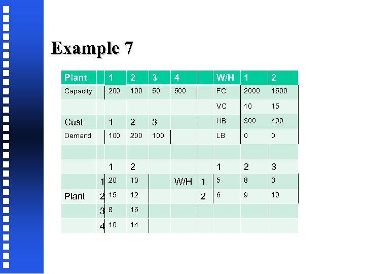Example 7 Plant 1 2 3 4 W/H 1 2 Capacity 200 100 50 500 FC 2000 1500 VC 10 15 Cust 1 2 3 UB 300 400 Demand 100 200 100 LB 0 0 1 2 3 1 20 10 W/H 1 5 8 3 2 15 12 2 6 9 10 3 8 16 4 10 14 Plant

Example 7 - MIP MODEL: [_1] MIN= 1000 * Y_1_1 + 2000 * Y_1_2 + 1000 * Y_1_3 + 1500 * Y_2_1 + 3000 * Y_2_2 + 1500 * Y_2_3 + 25 * X_1_1_1 + 28 * X_1_1_2 + 23 * X_1_1_3 + 16 * X_1_2_1 + 19 * X_1_2_2 + 20 * X_1_2_3 + 20 * X_2_1_1 + 23 * X_2_1_2 + 18 * X_2_1_3 + 18 * X_2_2_1 + 21 * X_2_2_2 + 22 * X_2_2_3 + 13 * X_3_1_1 + 16 * X_3_1_2 + 11 * X_3_1_3 + 22 * X_3_2_1 + 25 * X_3_2_2 + 26 * X_3_2_3 + 15 * X_4_1_1 + 18 * X_4_1_2 + 13 * X_4_1_3 + 20 * X_4_2_1 + 23 * X_4_2_2 + 24 * X_4_2_3 + 2000 * Z_1 + 1500 * Z_2 ; [_2] X_1_1_1 + X_1_1_2 + X_1_1_3 + X_1_2_1 + X_1_2_2 + X_1_2_3 <= 200 ; [_3] X_2_1_1 + X_2_1_2 + X_2_1_3 + X_2_2_1 + X_2_2_2 + X_2_2_3 <= 100 ; [_4] X_3_1_1 + X_3_1_2 + X_3_1_3 + X_3_2_1 + X_3_2_2 + X_3_2_3 <= 50 ; [_5] X_4_1_1 + X_4_1_2 + X_4_1_3 + X_4_2_1 + X_4_2_2 + X_4_2_3 <= 500 ; [_6] - 100 * Y_1_1 + X_1_1_1 + X_2_1_1 + X_3_1_1 + X_4_1_1 >= 0 ; [_7] - 200 * Y_1_2 + X_1_1_2 + X_2_1_2 + X_3_1_2 + X_4_1_2 >= 0 ; [_8] - 100 * Y_1_3 + X_1_1_3 + X_2_1_3 + X_3_1_3 + X_4_1_3 >= 0 ; [_9] - 100 * Y_2_1 + X_1_2_1 + X_2_2_1 + X_3_2_1 + X_4_2_1 >= 0 ; [_10] - 200 * Y_2_2 + X_1_2_2 + X_2_2_2 + X_3_2_2 + X_4_2_2 >= 0 ; [_11] - 100 * Y_2_3 + X_1_2_3 + X_2_2_3 + X_3_2_3 + X_4_2_3 >= 0 ; [_12] Y_1_1 + Y_2_1 = 1 ; [_13] Y_1_2 + Y_2_2 = 1 ; [_14] Y_1_3 + Y_2_3 = 1 ; [_15] 100 * Y_1_1 + 200 * Y_1_2 + 100 * Y_1_3 - 3000 * Z_1 <= 0 ; [_16] 100 * Y_2_1 + 200 * Y_2_2 + 100 * Y_2_3 - 4000 * Z_2 <= 0 ; [_17] 100 * Y_1_1 + 200 * Y_1_2 + 100 * Y_1_3 >= 0 ; [_18] 100 * Y_2_1 + 200 * Y_2_2 + 100 * Y_2_3 >= 0 ; @BIN( Y_1_1); @BIN( Y_1_2); @BIN( Y_1_3); @BIN( Y_2_1); @BIN( Y_2_2); @BIN( Y_2_3); @BIN( Z_1); @BIN( Z_2); END

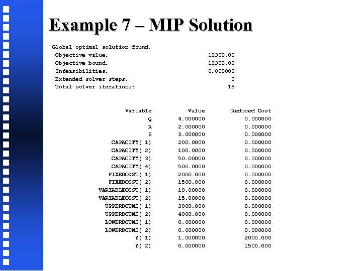Example 7 – MIP Solution Global optimal solution found. Objective value: 12300. 00 Objective bound: 12300. 00 Infeasibilities: 0. 000000 Extended solver steps: 0 Total solver iterations: 13 Variable Value Reduced Cost Q 4. 000000 0. 000000 R 2. 000000 0. 000000 S 3. 000000 0. 000000 CAPACITY( 1) 200. 0000 0. 000000 CAPACITY( 2) 100. 0000 0. 000000 CAPACITY( 3) 50. 00000 0. 000000 CAPACITY( 4) 500. 0000 0. 000000 FIXEDCOST( 1) 2000. 000 0. 000000 FIXEDCOST( 2) 1500. 000 0. 000000 VARIABLECOST( 1) 10. 00000 0. 000000 VARIABLECOST( 2) 15. 00000 0. 000000 UPPERBOUND( 1) 3000. 000 0. 000000 UPPERBOUND( 2) 4000. 000 0. 000000 LOWERBOUND( 1) 0. 000000 LOWERBOUND( 2) 0. 000000 Z( 1) 1. 000000 2000. 000 Z( 2) 0. 000000 1500. 000

Example 7 – LP MODEL: [_1] MIN= 25 * X_1_1_1 + 28 * X_1_1_2 + 23 * X_1_1_3 + 16 * X_1_2_1 + 19 * X_1_2_2 + 20 * X_1_2_3 + 20 * X_2_1_1 + 23 * X_2_1_2 + 18 * X_2_1_3 + 18 * X_2_2_1 + 21 * X_2_2_2 + 22 * X_2_2_3 + 13 * X_3_1_1 + 16 * X_3_1_2 + 11 * X_3_1_3 + 22 * X_3_2_1 + 25 * X_3_2_2 + 26 * X_3_2_3 + 15 * X_4_1_1 + 18 * X_4_1_2 + 13 * X_4_1_3 + 20 * X_4_2_1 + 23 * X_4_2_2 + 24 * X_4_2_3 + 7500 ; [_2] X_1_1_1 + X_1_1_2 + X_1_1_3 + X_1_2_1 + X_1_2_2 + X_1_2_3 <= 200 ; [_3] X_2_1_1 + X_2_1_2 + X_2_1_3 + X_2_2_1 + X_2_2_2 + X_2_2_3 <= 100 ; [_4] X_3_1_1 + X_3_1_2 + X_3_1_3 + X_3_2_1 + X_3_2_2 + X_3_2_3 <= 50 ; [_5] X_4_1_1 + X_4_1_2 + X_4_1_3 + X_4_2_1 + X_4_2_2 + X_4_2_3 <= 500 ; [_6] X_1_1_1 + X_2_1_1 + X_3_1_1 + X_4_1_1 >= 0 ; [_7] X_1_1_2 + X_2_1_2 + X_3_1_2 + X_4_1_2 >= 0 ; [_8] X_1_1_3 + X_2_1_3 + X_3_1_3 + X_4_1_3 >= 0 ; [_9] X_1_2_1 + X_2_2_1 + X_3_2_1 + X_4_2_1 >= 100 ; [_10] X_1_2_2 + X_2_2_2 + X_3_2_2 + X_4_2_2 >= 200 ; [_11] X_1_2_3 + X_2_2_3 + X_3_2_3 + X_4_2_3 >= 100 ; [_12] 0 = 0 ; [_13] 0 = 0 ; [_14] 0 = 0 ; [_15] 0 <= 0 ; [_16] 0 <= 3600 ; [_17] 0 >= 0 ; [_18] 0 >= - 400 ; END

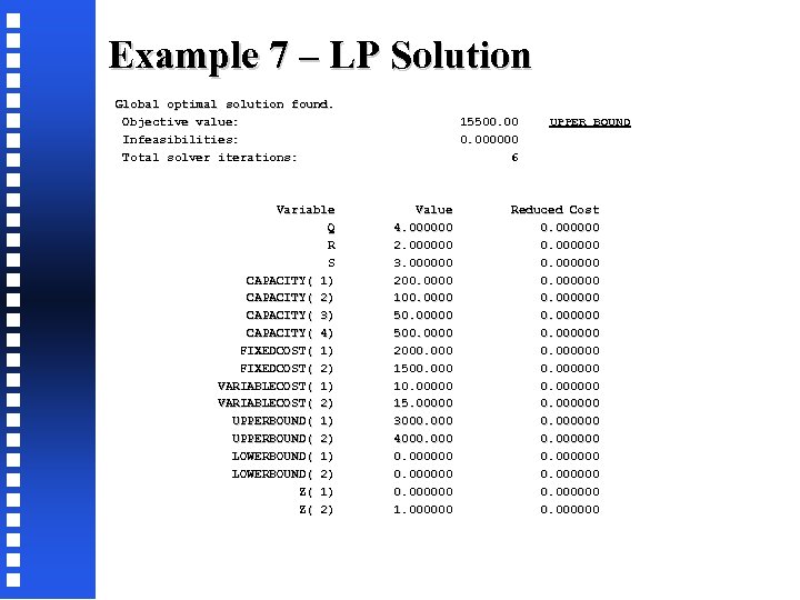Example 7 – LP Solution Global optimal solution found. Objective value: 15500. 00 UPPER BOUND Infeasibilities: 0. 000000 Total solver iterations: 6 Variable Value Reduced Cost Q 4. 000000 0. 000000 R 2. 000000 0. 000000 S 3. 000000 0. 000000 CAPACITY( 1) 200. 0000 0. 000000 CAPACITY( 2) 100. 0000 0. 000000 CAPACITY( 3) 50. 00000 0. 000000 CAPACITY( 4) 500. 0000 0. 000000 FIXEDCOST( 1) 2000. 000 0. 000000 FIXEDCOST( 2) 1500. 000 0. 000000 VARIABLECOST( 1) 10. 00000 0. 000000 VARIABLECOST( 2) 15. 00000 0. 000000 UPPERBOUND( 1) 3000. 000 0. 000000 UPPERBOUND( 2) 4000. 000 0. 000000 LOWERBOUND( 1) 0. 000000 LOWERBOUND( 2) 0. 000000 Z( 1) 0. 000000 Z( 2) 1. 000000 0. 000000

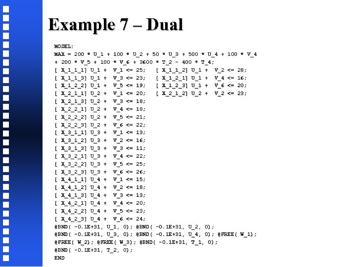Example 7 – Dual MODEL: MAX = 200 * U_1 + 100 * U_2 + 50 * U_3 + 500 * U_4 + 100 * V_4 + 200 * V_5 + 100 * V_6 + 3600 * T_2 - 400 * T_4; [ X_1_1_1] U_1 + V_1 <= 25; [ X_1_1_2] U_1 + V_2 <= 28; [ X_1_1_3] U_1 + V_3 <= 23; [ X_1_2_1] U_1 + V_4 <= 16; [ X_1_2_2] U_1 + V_5 <= 19; [ X_1_2_3] U_1 + V_6 <= 20; [ X_2_1_1] U_2 + V_1 <= 20; [ X_2_1_2] U_2 + V_2 <= 23; [ X_2_1_3] U_2 + V_3 <= 18; [ X_2_2_1] U_2 + V_4 <= 18; [ X_2_2_2] U_2 + V_5 <= 21; [ X_2_2_3] U_2 + V_6 <= 22; [ X_3_1_1] U_3 + V_1 <= 13; [ X_3_1_2] U_3 + V_2 <= 16; [ X_3_1_3] U_3 + V_3 <= 11; [ X_3_2_1] U_3 + V_4 <= 22; [ X_3_2_2] U_3 + V_5 <= 25; [ X_3_2_3] U_3 + V_6 <= 26; [ X_4_1_1] U_4 + V_1 <= 15; [ X_4_1_2] U_4 + V_2 <= 18; [ X_4_1_3] U_4 + V_3 <= 13; [ X_4_2_1] U_4 + V_4 <= 20; [ X_4_2_2] U_4 + V_5 <= 23; [ X_4_2_3] U_4 + V_6 <= 24; @BND( -0. 1 E+31, U_1, 0); @BND( -0. 1 E+31, U_2, 0); @BND( -0. 1 E+31, U_3, 0); @BND( -0. 1 E+31, U_4, 0); @FREE( W_1); @FREE( W_2); @FREE( W_3); @BND( -0. 1 E+31, T_1, 0); @BND( -0. 1 E+31, T_2, 0); END

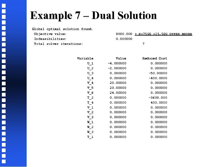Example 7 – Dual Solution Global optimal solution found. Objective value: 8000. 000 + K=7500 =15, 500 UPPER BOUND Infeasibilities: 0. 000000 Total solver iterations: 7 Variable Value Reduced Cost U_1 -4. 000000 0. 000000 U_2 -2. 000000 0. 000000 U_3 0. 000000 -50. 00000 U_4 0. 000000 -400. 0000 V_4 20. 00000 0. 000000 V_5 23. 00000 0. 000000 V_6 24. 00000 0. 000000 T_2 0. 000000 -3600. 000 T_4 0. 000000 400. 0000 V_1 0. 000000 V_2 0. 000000 V_3 0. 000000 W_1 0. 000000 W_2 0. 000000 W_3 0. 000000 T_1 0. 000000

Example 7 – Master Problem MODEL: [_1] MIN= Z; [_2] Z >= -1000 + 2000 * Y_2_1 + 4600 * Y_2_2 + 2400 * Y_2_3 + 1000 * Y_1_1 + 2000 * Y_1_2 + 1000 * Y_1_3 + 1500 * Y_2_1 + 3000 * Y_2_2 + 1500 * Y_2_3 + 2000 * Z_1 + 1500 * Z_2 ; [_4] - 100 * Y_1_1 + X_1_1_1 + X_2_1_1 + X_3_1_1 + X_4_1_1 >= 0 ; [_5] - 200 * Y_1_2 + X_1_1_2 + X_2_1_2 + X_3_1_2 + X_4_1_2 >= 0 ; [_6] - 100 * Y_1_3 + X_1_1_3 + X_2_1_3 + X_3_1_3 + X_4_1_3 >= 0 ; [_7] - 100 * Y_2_1 + X_1_2_1 + X_2_2_1 + X_3_2_1 + X_4_2_1 >= 0 ; [_8] - 200 * Y_2_2 + X_1_2_2 + X_2_2_2 + X_3_2_2 + X_4_2_2 >= 0 ; [_9] - 100 * Y_2_3 + X_1_2_3 + X_2_2_3 + X_3_2_3 + X_4_2_3 >= 0 ; [_10] Y_1_1 + Y_2_1 = 1 ; [_11] Y_1_2 + Y_2_2 = 1 ; [_12] Y_1_3 + Y_2_3 = 1 ; [_13] 100 * Y_1_1 + 200 * Y_1_2 + 100 * Y_1_3 - 3000 * Z_1 <= 0 ; [_14] 100 * Y_2_1 + 200 * Y_2_2 + 100 * Y_2_3 - 4000 * Z_2 <= 0 ; [_15] 100 * Y_1_1 + 200 * Y_1_2 + 100 * Y_1_3 >= 0 ; [_16] 100 * Y_2_1 + 200 * Y_2_2 + 100 * Y_2_3 >= 0 ; @BIN( Y_1_1); @BIN( Y_1_2); @BIN( Y_1_3); @BIN( Y_2_1); @BIN( Y_2_2); @BIN( Y_2_3); @BIN( Z_1); @BIN( Z_2); END

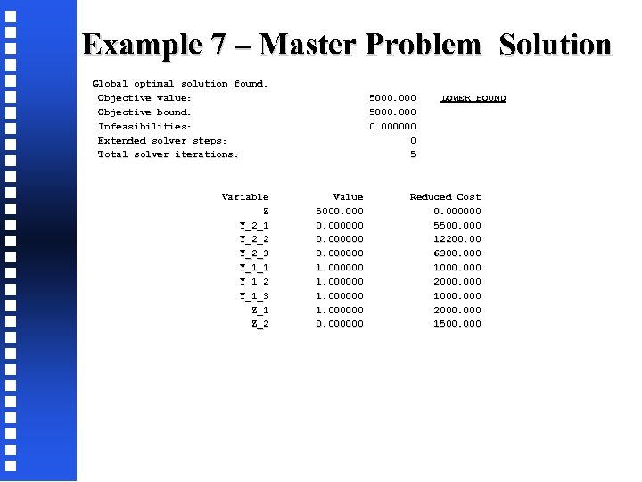Example 7 – Master Problem Solution Global optimal solution found. Objective value: 5000. 000 LOWER BOUND Objective bound: 5000. 000 Infeasibilities: 0. 000000 Extended solver steps: 0 Total solver iterations: 5 Variable Value Reduced Cost Z 5000. 000 0. 000000 Y_2_1 0. 000000 5500. 000 Y_2_2 0. 000000 12200. 00 Y_2_3 0. 000000 6300. 000 Y_1_1 1. 000000 1000. 000 Y_1_2 1. 000000 2000. 000 Y_1_3 1. 000000 1000. 000 Z_1 1. 000000 2000. 000 Z_2 0. 000000 1500. 000

Example 7 – LP MODEL: [_1] MIN= 25 * X_1_1_1 + 28 * X_1_1_2 + 23 * X_1_1_3 + 16 * X_1_2_1 + 19 * X_1_2_2 + 20 * X_1_2_3 + 20 * X_2_1_1 + 23 * X_2_1_2 + 18 * X_2_1_3 + 18 * X_2_2_1 + 21 * X_2_2_2 + 22 * X_2_2_3 + 13 * X_3_1_1 + 16 * X_3_1_2 + 11 * X_3_1_3 + 22 * X_3_2_1 + 25 * X_3_2_2 + 26 * X_3_2_3 + 15 * X_4_1_1 + 18 * X_4_1_2 + 13 * X_4_1_3 + 20 * X_4_2_1 + 23 * X_4_2_2 + 24 * X_4_2_3 + 6000 ; [_2] X_1_1_1 + X_1_1_2 + X_1_1_3 + X_1_2_1 + X_1_2_2 + X_1_2_3 <= 200 ; [_3] X_2_1_1 + X_2_1_2 + X_2_1_3 + X_2_2_1 + X_2_2_2 + X_2_2_3 <= 100 ; [_4] X_3_1_1 + X_3_1_2 + X_3_1_3 + X_3_2_1 + X_3_2_2 + X_3_2_3 <= 50 ; [_5] X_4_1_1 + X_4_1_2 + X_4_1_3 + X_4_2_1 + X_4_2_2 + X_4_2_3 <= 500 ; [_6] X_1_1_1 + X_2_1_1 + X_3_1_1 + X_4_1_1 >= 100 ; [_7] X_1_1_2 + X_2_1_2 + X_3_1_2 + X_4_1_2 >= 200 ; [_8] X_1_1_3 + X_2_1_3 + X_3_1_3 + X_4_1_3 >= 100 ; [_9] X_1_2_1 + X_2_2_1 + X_3_2_1 + X_4_2_1 >= 0 ; [_10] X_1_2_2 + X_2_2_2 + X_3_2_2 + X_4_2_2 >= 0 ; [_11] X_1_2_3 + X_2_2_3 + X_3_2_3 + X_4_2_3 >= 0 ; [_12] 0 = 0 ; [_13] 0 = 0 ; [_14] 0 = 0 ; [_15] 0 <= 2600 ; [_16] 0 <= 0 ; [_17] 0 >= - 400 ; [_18] 0 >= 0 ; END

Example 7 – LP Solution Global optimal solution found. Objective value: 12300. 00 UPPER BOUND Infeasibilities: 0. 000000 Total solver iterations: 6 Variable Value Reduced Cost Q 4. 000000 0. 000000 R 2. 000000 0. 000000 S 3. 000000 0. 000000 CAPACITY( 1) 200. 0000 0. 000000 CAPACITY( 2) 100. 0000 0. 000000 CAPACITY( 3) 50. 00000 0. 000000 CAPACITY( 4) 500. 0000 0. 000000 FIXEDCOST( 1) 2000. 000 0. 000000 FIXEDCOST( 2) 1500. 000 0. 000000 VARIABLECOST( 1) 10. 00000 0. 000000 VARIABLECOST( 2) 15. 00000 0. 000000 UPPERBOUND( 1) 3000. 000 0. 000000 UPPERBOUND( 2) 4000. 000 0. 000000 LOWERBOUND( 1) 0. 000000 LOWERBOUND( 2) 0. 000000 Z( 1) 1. 000000 0. 000000 Z( 2) 0. 000000

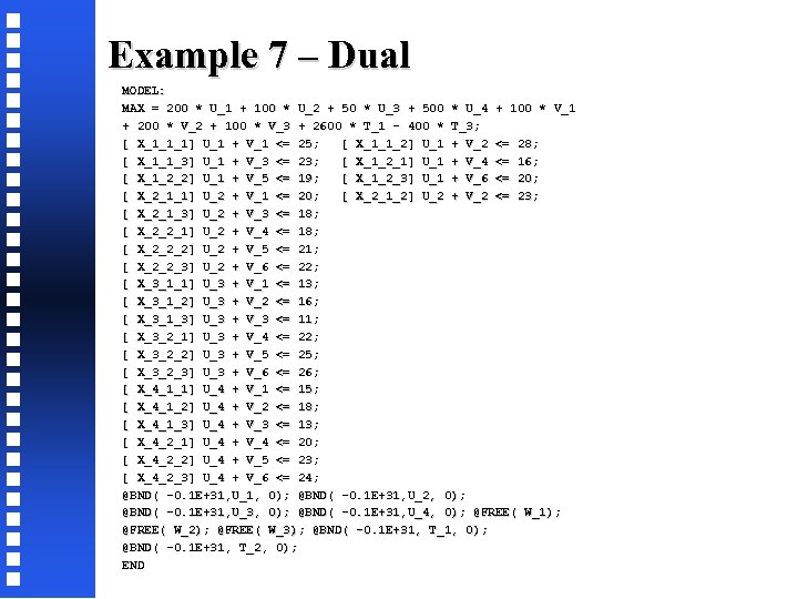Example 7 – Dual MODEL: MAX = 200 * U_1 + 100 * U_2 + 50 * U_3 + 500 * U_4 + 100 * V_1 + 200 * V_2 + 100 * V_3 + 2600 * T_1 - 400 * T_3; [ X_1_1_1] U_1 + V_1 <= 25; [ X_1_1_2] U_1 + V_2 <= 28; [ X_1_1_3] U_1 + V_3 <= 23; [ X_1_2_1] U_1 + V_4 <= 16; [ X_1_2_2] U_1 + V_5 <= 19; [ X_1_2_3] U_1 + V_6 <= 20; [ X_2_1_1] U_2 + V_1 <= 20; [ X_2_1_2] U_2 + V_2 <= 23; [ X_2_1_3] U_2 + V_3 <= 18; [ X_2_2_1] U_2 + V_4 <= 18; [ X_2_2_2] U_2 + V_5 <= 21; [ X_2_2_3] U_2 + V_6 <= 22; [ X_3_1_1] U_3 + V_1 <= 13; [ X_3_1_2] U_3 + V_2 <= 16; [ X_3_1_3] U_3 + V_3 <= 11; [ X_3_2_1] U_3 + V_4 <= 22; [ X_3_2_2] U_3 + V_5 <= 25; [ X_3_2_3] U_3 + V_6 <= 26; [ X_4_1_1] U_4 + V_1 <= 15; [ X_4_1_2] U_4 + V_2 <= 18; [ X_4_1_3] U_4 + V_3 <= 13; [ X_4_2_1] U_4 + V_4 <= 20; [ X_4_2_2] U_4 + V_5 <= 23; [ X_4_2_3] U_4 + V_6 <= 24; @BND( -0. 1 E+31, U_1, 0); @BND( -0. 1 E+31, U_2, 0); @BND( -0. 1 E+31, U_3, 0); @BND( -0. 1 E+31, U_4, 0); @FREE( W_1); @FREE( W_2); @FREE( W_3); @BND( -0. 1 E+31, T_1, 0); @BND( -0. 1 E+31, T_2, 0); END

Example 7 – Dual Solution Global optimal solution found. Objective value: 6300. 000 + K = 6000 = 12300 UPPPER BOUND Infeasibilities: 0. 000000 Total solver iterations: 10 Variable Value Reduced Cost U_1 0. 000000 -200. 0000 U_2 0. 000000 -100. 0000 U_3 -2. 000000 0. 000000 U_4 0. 000000 -150. 0000 V_1 15. 00000 0. 000000 V_2 18. 00000 0. 000000 V_3 13. 00000 0. 000000 T_1 0. 000000 -2600. 000 T_3 0. 000000 400. 0000 V_4 0. 000000 V_5 0. 000000 V_6 0. 000000 W_1 0. 000000 W_2 0. 000000 W_3 0. 000000 T_2 0. 000000

Example 7 – Master Problem MODEL: [_1] MIN= Z; [_2] Z >= -1000 + 2000 * Y_2_1 + 4600 * Y_2_2 + 2400 * Y_2_3 + 1000 * Y_1_1 + 2000 * Y_1_2 + 1000 * Y_1_3 + 1500 * Y_2_1 + 3000 * Y_2_2 + 1500 * Y_2_3 + 2000 * Z_1 + 1500 * Z_2 ; [_3] Z >= -100 + 1500 * Y_1_1 + 3600 * Y_1_2 + 1300 * Y_1_3 + 1000 * Y_1_1 + 2000 * Y_1_2 + 1000 * Y_1_3 + 1500 * Y_2_1 + 3000 * Y_2_2 + 1500 * Y_2_3 + 2000 * Z_1 + 1500 * Z_2 ; [_4] - 100 * Y_1_1 + X_1_1_1 + X_2_1_1 + X_3_1_1 + X_4_1_1 >= 0 ; [_5] - 200 * Y_1_2 + X_1_1_2 + X_2_1_2 + X_3_1_2 + X_4_1_2 >= 0 ; [_6] - 100 * Y_1_3 + X_1_1_3 + X_2_1_3 + X_3_1_3 + X_4_1_3 >= 0 ; [_7] - 100 * Y_2_1 + X_1_2_1 + X_2_2_1 + X_3_2_1 + X_4_2_1 >= 0 ; [_8] - 200 * Y_2_2 + X_1_2_2 + X_2_2_2 + X_3_2_2 + X_4_2_2 >= 0 ; [_9] - 100 * Y_2_3 + X_1_2_3 + X_2_2_3 + X_3_2_3 + X_4_2_3 >= 0 ; [_10] Y_1_1 + Y_2_1 = 1 ; [_11] Y_1_2 + Y_2_2 = 1 ; [_12] Y_1_3 + Y_2_3 = 1 ; [_13] 100 * Y_1_1 + 200 * Y_1_2 + 100 * Y_1_3 - 3000 * Z_1 <= 0 ; [_14] 100 * Y_2_1 + 200 * Y_2_2 + 100 * Y_2_3 - 4000 * Z_2 <= 0 ; [_15] 100 * Y_1_1 + 200 * Y_1_2 + 100 * Y_1_3 >= 0 ; [_16] 100 * Y_2_1 + 200 * Y_2_2 + 100 * Y_2_3 >= 0 ; @BIN( Y_1_1); @BIN( Y_1_2); @BIN( Y_1_3); @BIN( Y_2_1); @BIN( Y_2_2); @BIN( Y_2_3); @BIN( Z_1); @BIN( Z_2); END

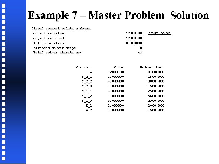Example 7 – Master Problem Solution Global optimal solution found. Objective value: 12000. 00 LOWER BOUND Objective bound: 12000. 00 Infeasibilities: 0. 000000 Extended solver steps: 0 Total solver iterations: 43 Variable Value Reduced Cost Z 12000. 00 0. 000000 Y_2_1 1. 000000 1500. 000 Y_2_2 0. 000000 3000. 000 Y_2_3 1. 000000 1500. 000 Y_1_1 0. 000000 2500. 000 Y_1_2 1. 000000 5600. 000 Y_1_3 0. 000000 2300. 000 Z_1 1. 000000 2000. 000 Z_2 1. 000000 1500. 000

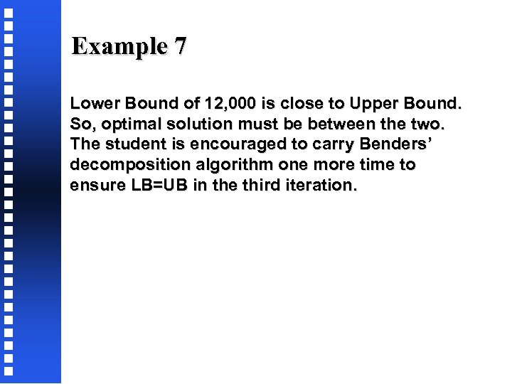Example 7 Lower Bound of 12, 000 is close to Upper Bound. So, optimal solution must be between the two. The student is encouraged to carry Benders’ decomposition algorithm one more time to ensure LB=UB in the third iteration.