f MRI Quality Assurance QA v 2 Data

f. MRI Quality Assurance (QA) (v 2) Data acquisition, processing and analysis Katherine Lymer Medical Physicist in MR Support SFC Brain Imaging Research Centre for Scotland, University of Edinburgh

f. MRI QA: Objectives • Describe the quality of the f. MRI data Using measures of SNR, SFNR, fluctuation and drift • Monitor the long-term stability of scanner performance in f. MRI • Allow between site-assessments of f. MRI data

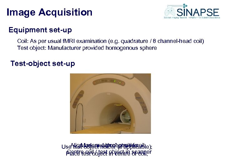Image Acquisition Equipment set-up Coil: As per usual f. MRI examination (e. g. quadrature / 8 channel-head coil) Test object: Manufacturer provided homogenous sphere Test-object set-up Align lasers with centre of coil; Mark as “zero” position Use test object holder (if applicable); Centre coil / test object in of coil; Place test object in centre scanner

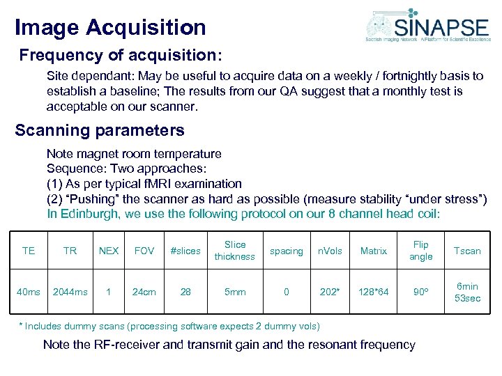Image Acquisition Frequency of acquisition: Site dependant: May be useful to acquire data on a weekly / fortnightly basis to establish a baseline; The results from our QA suggest that a monthly test is acceptable on our scanner. Scanning parameters Note magnet room temperature Sequence: Two approaches: (1) As per typical f. MRI examination (2) “Pushing” the scanner as hard as possible (measure stability “under stress”) In Edinburgh, we use the following protocol on our 8 channel head coil: TE TR NEX FOV #slices Slice thickness spacing n. Vols Matrix Flip angle Tscan 40 ms 2044 ms 1 24 cm 28 5 mm 0 202* 128*64 90º 6 min 53 sec * Includes dummy scans (processing software expects 2 dummy vols) Note the RF-receiver and transmit gain and the resonant frequency

Image Processing Transfer data to “off-line” to image analysis work station NB This processing protocol is based upon that provided by the BIRN (http: //www. nbirn. net/research/function/fbirn_tools_primer. shtm) and is similar to that used in “Calibrain”. See also: Weisskoff et al, MRM 36: 643 -645, 1996 Friedman et al, JMRI 23: 827– 839, 2006 Requirements: (1) PC / workstation with matlab; (2) SPM 5 (as supplied by the FIL: http: //www. fil. ion. ucl. ac. uk/spm/) (3) f. MRI_qa. m script (as supplied by f. BIRN: http: //www-calit 2. nbirn. net/tools/fbirn_stability_phantom/index. shtm) This script needs to be modified to reflect local / in-house needs (4) mricro

Data Management (1) Ensure that data is stored in central f. MRI data store, in appropriate folder denoting the current QA session (E. g. In Edinburgh, the data is stored in Y: MONTHLY_QA using the format: QAddmmyyyy. TEMPtt_yyyymmdd_study. Number) (2) In the relevant monthly QA folder, make two new sub-folders to differenentiate between the raw and reconstructed data e. g. “raw_data” and “SPM 5_output”. (3) Copy the f. MRI dicom files into the raw_data folder (4) (E. g. in Edinburgh, this is: QAddmmyyyy. TEMPtt_yyyymmdd_study. Numberraw_data)

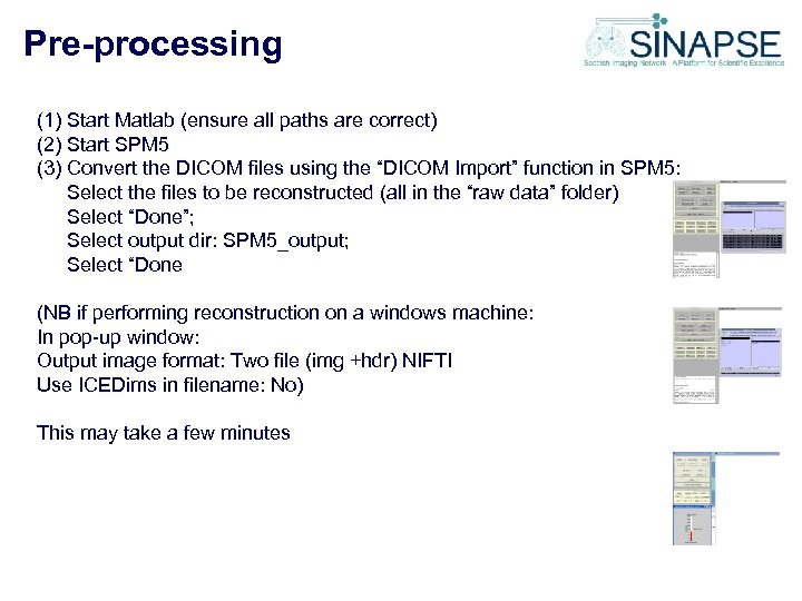Pre-processing (1) Start Matlab (ensure all paths are correct) (2) Start SPM 5 (3) Convert the DICOM files using the “DICOM Import” function in SPM 5: Select the files to be reconstructed (all in the “raw data” folder) Select “Done”; Select output dir: SPM 5_output; Select “Done (NB if performing reconstruction on a windows machine: In pop-up window: Output image format: Two file (img +hdr) NIFTI Use ICEDims in filename: No) This may take a few minutes

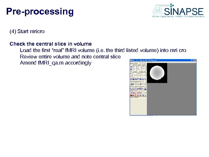Pre-processing (4) Start mricro Check the central slice in volume Load the first “real” f. MRI volume (i. e. the third listed volume) into mri cro Review entire volume and note central slice Amend f. MRI_qa. m accordingly

Image Processing: f. MRI_qa_calc Edits required to f. MRI_qa (original version obtained from http: //wwwcalit 2. nbirn. net/tools/fbirn_stability_phantom/index. shtm) (1) Ensure TR is correct; (2) Ensure that the date is in the correct format; (3) Define dimensions of ROI for ghosting measurement by changing: X 1 G, X 2 G, Y 1 G, Y 2 G (4) Ensure that the central ROI is placed appropriately within the central image (5) Check that the central slice number is correct (i. e. it matches that practically acquired)

Image Processing: f. MRI_qa_calc Run your version of f. MRI_qa Import values into excel spreadsheet; Plot results to help identify any trends / outliers. Note any variation in RF-receiver / -transmit gain and resonant frequency (since the phantom and the protocol remain the same, these should remain constant)

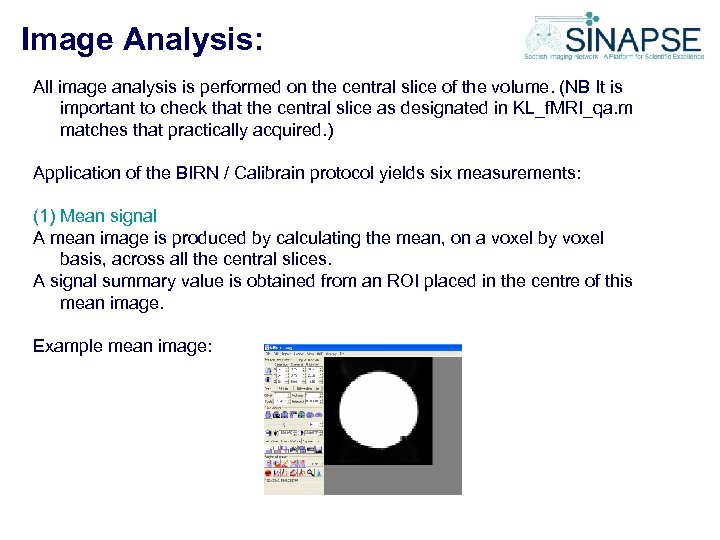Image Analysis: All image analysis is performed on the central slice of the volume. (NB It is important to check that the central slice as designated in KL_f. MRI_qa. m matches that practically acquired. ) Application of the BIRN / Calibrain protocol yields six measurements: (1) Mean signal A mean image is produced by calculating the mean, on a voxel by voxel basis, across all the central slices. A signal summary value is obtained from an ROI placed in the centre of this mean image. Example mean image:

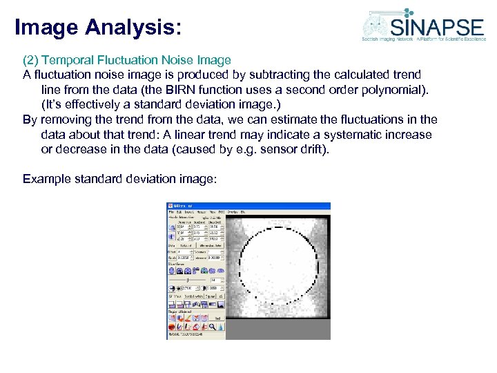Image Analysis: (2) Temporal Fluctuation Noise Image A fluctuation noise image is produced by subtracting the calculated trend line from the data (the BIRN function uses a second order polynomial). (It’s effectively a standard deviation image. ) By removing the trend from the data, we can estimate the fluctuations in the data about that trend: A linear trend may indicate a systematic increase or decrease in the data (caused by e. g. sensor drift). Example standard deviation image:

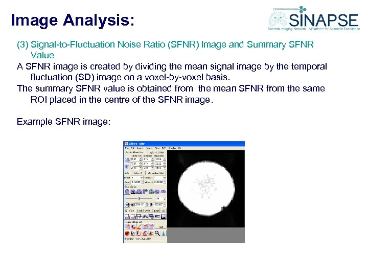Image Analysis: (3) Signal-to-Fluctuation Noise Ratio (SFNR) Image and Summary SFNR Value A SFNR image is created by dividing the mean signal image by the temporal fluctuation (SD) image on a voxel-by-voxel basis. The summary SFNR value is obtained from the mean SFNR from the same ROI placed in the centre of the SFNR image. Example SFNR image:

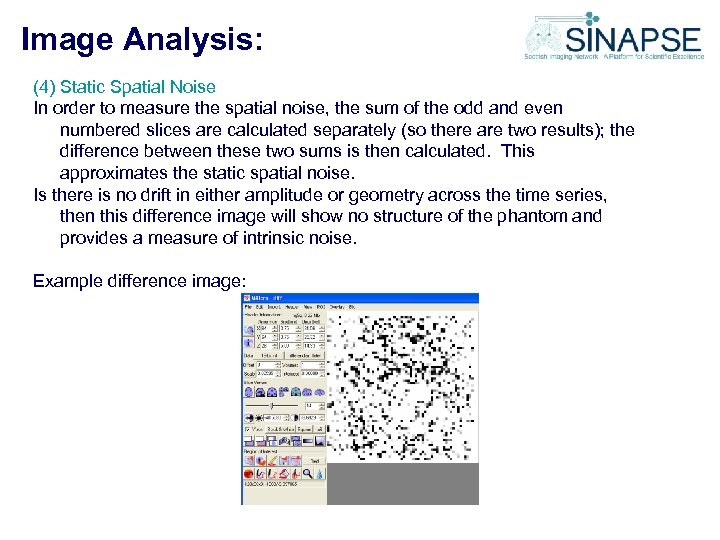Image Analysis: (4) Static Spatial Noise In order to measure the spatial noise, the sum of the odd and even numbered slices are calculated separately (so there are two results); the difference between these two sums is then calculated. This approximates the static spatial noise. Is there is no drift in either amplitude or geometry across the time series, then this difference image will show no structure of the phantom and provides a measure of intrinsic noise. Example difference image:

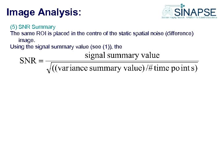Image Analysis: (5) SNR Summary The same ROI is placed in the centre of the static spatial noise (difference) image. Using the signal summary value (see (1)), the

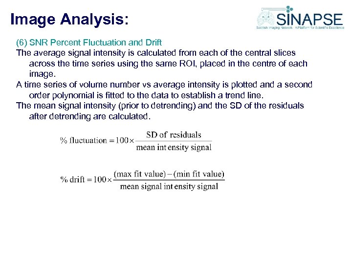Image Analysis: (6) SNR Percent Fluctuation and Drift The average signal intensity is calculated from each of the central slices across the time series using the same ROI, placed in the centre of each image. A time series of volume number vs average intensity is plotted and a second order polynomial is fitted to the data to establish a trend line. The mean signal intensity (prior to detrending) and the SD of the residuals after detrending are calculated.

Image Analysis: (7) Summary graphs In addition, a series of summary graphs showing the change in raw signal, SGR, magnitude spectrum and relative standard deviation will be displayed

Image Analysis: (8) Signal-to-Ghost Ratio (SGR) In addition to the BIRN tests, a signal to ghost (SGR) measurement was added to the protocol by Dr Gordon Waiter, Aberdeen Biomedical Imaging Centre, University of Aberdeen. The image may have to be windowed to observe the ghost. In order to make the SGR measurement, a second (ghosting) ROI is defined within the ghosting region of the image. The SGR summary value is calculated from the mean signal (from the central ROI) / mean signal (from the ghosting ROI).

SINAPSE Reporting Mechanism: Short-term Maintain results locally; Distribute summary results with colleagues e. g. for multi-centre studies, comparisons of scanner performance (KL happy to hold central data base and distribute as required). Medium - Long term We aim to produce a SINAPSE QA reporting website to which these results can be uploaded. Watch this space…………. . !