F 4 Large Scale Automated Forecasting Using Fractals

F 4: Large Scale Automated Forecasting Using Fractals -Deepayan Chakrabarti -Christos Faloutsos Deepayan Chakrabarti CIKM 2002 1

Outline n n Introduction/Motivation Survey and Lag Plots Exact Problem Formulation Proposed Method n n Fractal Dimensions Background Our method Results Conclusions Deepayan Chakrabarti CIKM 2002 2

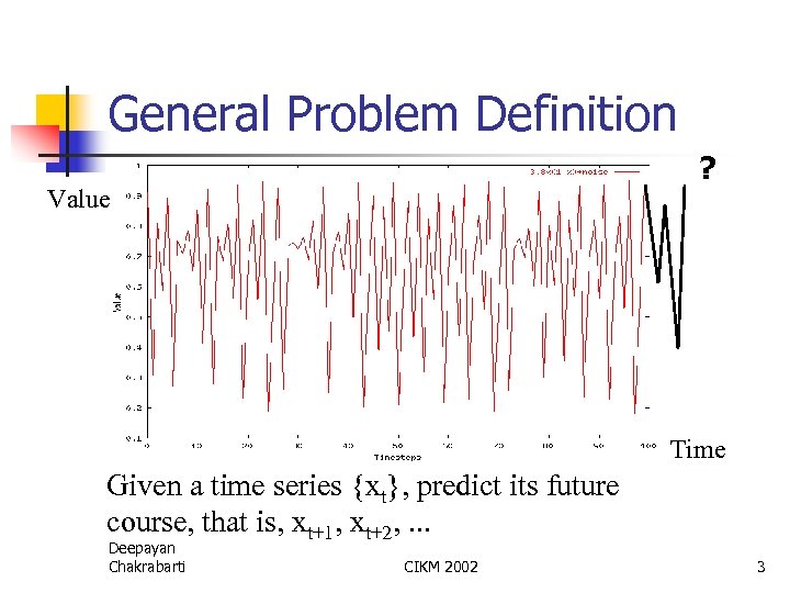General Problem Definition ? Value Time Given a time series {xt}, predict its future course, that is, xt+1, xt+2, . . . Deepayan Chakrabarti CIKM 2002 3

Motivation Traditional fields • Financial data analysis • Physiological data, elderly care • Weather, environmental studies Sensor Networks (MEMS, “Smart. Dust”) • Long / “infinite” series • No human intervention “black box” Deepayan Chakrabarti CIKM 2002 4

Outline n n Introduction/Motivation Survey and Lag Plots Exact Problem Formulation Proposed Method n n Fractal Dimensions Background Our method Results Conclusions Deepayan Chakrabarti CIKM 2002 5

How to forecast? ARIMA but linearity assumption n Neural Networks but large number of parameters and long training times [Wan/1993, Mozer/1993] n Hidden Markov Models O(N 2) in number of nodes N; also fixing N is a problem [Ge+/2000] µ Lag Plots n Deepayan Chakrabarti CIKM 2002 6

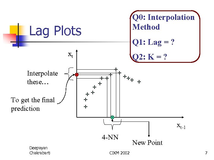Q 0: Interpolation Method Lag Plots Q 1: Lag = ? xt Q 2: K = ? Interpolate these… To get the final prediction xt-1 4 -NN Deepayan Chakrabarti CIKM 2002 New Point 7

Q 0: Interpolation Using SVD (state of the art) [Sauer/1993] xt Deepayan Chakrabarti Xt-1 CIKM 2002 8

Why Lag Plots? n n Based on the “Takens’ Theorem” [Takens/1981] which says that delay vectors can be used for predictive purposes Deepayan Chakrabarti CIKM 2002 9

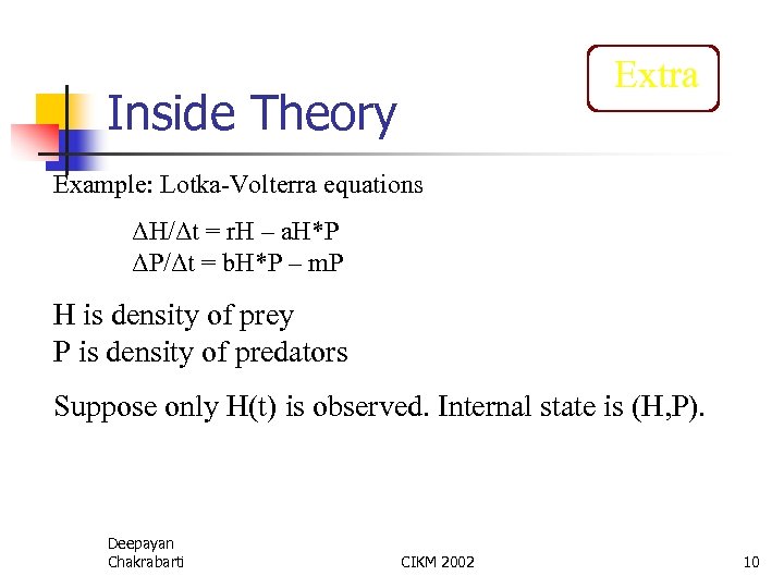Extra Inside Theory Example: Lotka-Volterra equations ΔH/Δt = r. H – a. H*P ΔP/Δt = b. H*P – m. P H is density of prey P is density of predators Suppose only H(t) is observed. Internal state is (H, P). Deepayan Chakrabarti CIKM 2002 10

Outline n n Introduction/Motivation Survey and Lag Plots Exact Problem Formulation Proposed Method n n Fractal Dimensions Background Our method Results Conclusions Deepayan Chakrabarti CIKM 2002 11

Problem at hand Given {x 1, x 2, …, x. N} F Automatically set parameters - L(opt) (from Q 1) - k(opt) (from Q 2) F in Linear time on N F to minimise Normalized Mean Squared Error (NMSE) of forecasting F Deepayan Chakrabarti CIKM 2002 12

Previous work/Alternatives n n n Manual Setting : BUT infeasible [Sauer/1992] Cross. Validation : BUT Slow; leave-oneout crossvalidation ~ O(N 2 log. N) or more “False Nearest Neighbors” : BUT Unstable [Abarbanel/1996] Deepayan Chakrabarti CIKM 2002 13

Outline n n Introduction/Motivation Survey and Lag Plots Exact Problem Formulation Proposed Method n n Fractal Dimensions Background Our method Results Conclusions Deepayan Chakrabarti CIKM 2002 14

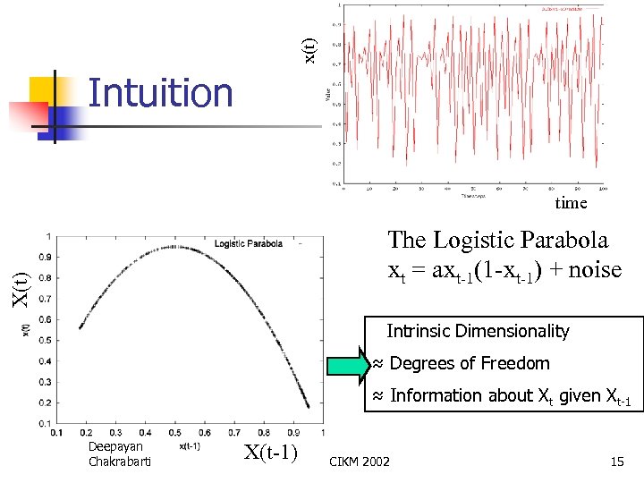x(t) Intuition time X(t) The Logistic Parabola xt = axt-1(1 -xt-1) + noise Intrinsic Dimensionality ≈ Degrees of Freedom ≈ Information about Xt given Xt-1 Deepayan Chakrabarti X(t-1) CIKM 2002 15

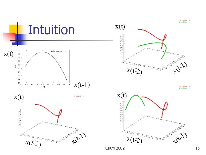Intuition x(t) x(t-2) -1) x(t-1) x(t) x(t-2) x -1) (t x(t-2) CIKM 2002 -1) x(t 16

Intuition n To find L(opt): n n Go further back in time (ie. , consider Xt-2, Xt-3 and so on) Till there is no more information gained about Xt Deepayan Chakrabarti CIKM 2002 17

Outline n n Introduction/Motivation Survey and Lag Plots Exact Problem Formulation Proposed Method n n Fractal Dimensions Background Our method Results Conclusions Deepayan Chakrabarti CIKM 2002 18

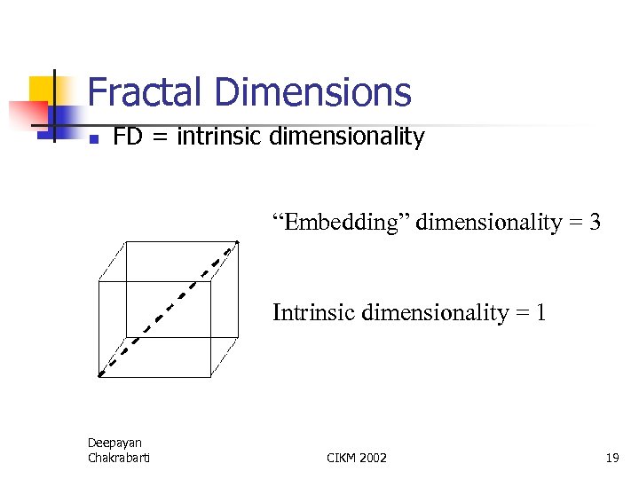Fractal Dimensions n FD = intrinsic dimensionality “Embedding” dimensionality = 3 Intrinsic dimensionality = 1 Deepayan Chakrabarti CIKM 2002 19

FD Fractal dimensionality = intrinsic Dimensions [Belussi/1995] log( # pairs) Points to note: • FD can be a noninteger • There are fast methods to compute it Deepayan Chakrabarti CIKM 2002 log(r) 20

Outline n n Introduction/Motivation Survey and Lag Plots Exact Problem Formulation Proposed Method n n Fractal Dimensions Background Our method Results Conclusions Deepayan Chakrabarti CIKM 2002 21

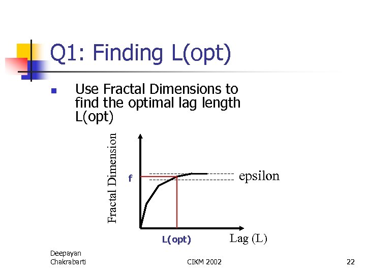Q 1: Finding L(opt) Use Fractal Dimensions to find the optimal lag length L(opt) Fractal Dimension n epsilon f L(opt) Deepayan Chakrabarti CIKM 2002 Lag (L) 22

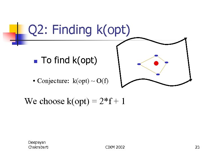Q 2: Finding k(opt) n To find k(opt) • Conjecture: k(opt) ~ O(f) We choose k(opt) = 2*f + 1 Deepayan Chakrabarti CIKM 2002 23

Outline n n Introduction/Motivation Survey and Lag Plots Exact Problem Formulation Proposed Method n n Fractal Dimensions Background Our method Results Conclusions Deepayan Chakrabarti CIKM 2002 24

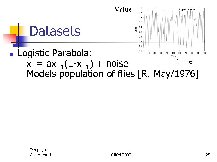Value Datasets n Logistic Parabola: Time xt = axt-1(1 -xt-1) + noise Models population of flies [R. May/1976] Deepayan Chakrabarti CIKM 2002 25

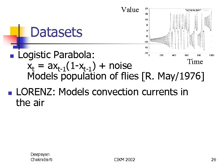Value Datasets n n Logistic Parabola: Time xt = axt-1(1 -xt-1) + noise Models population of flies [R. May/1976] LORENZ: Models convection currents in the air Deepayan Chakrabarti CIKM 2002 26

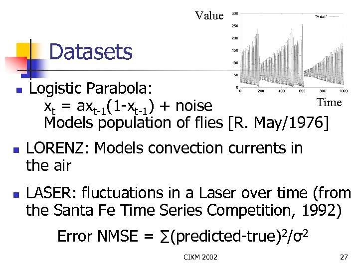Value Datasets n n n Logistic Parabola: Time xt = axt-1(1 -xt-1) + noise Models population of flies [R. May/1976] LORENZ: Models convection currents in the air LASER: fluctuations in a Laser over time (from the Santa Fe Time Series Competition, 1992) Error NMSE = ∑(predicted-true)2/σ2 CIKM 2002 27

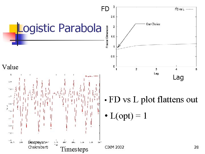FD Logistic Parabola Value Lag • FD vs L plot flattens out • L(opt) = 1 Deepayan Chakrabarti Timesteps CIKM 2002 28

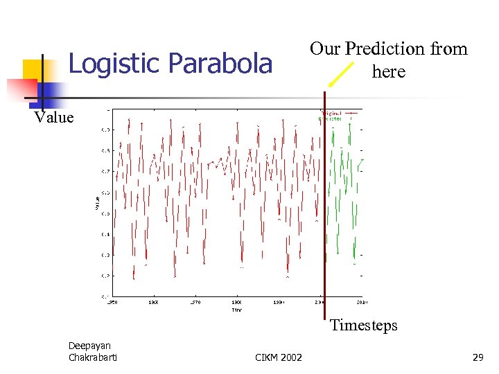Logistic Parabola Our Prediction from here Value Timesteps Deepayan Chakrabarti CIKM 2002 29

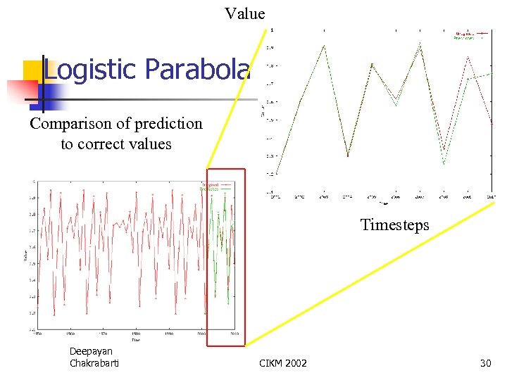Value Logistic Parabola Comparison of prediction to correct values Timesteps Deepayan Chakrabarti CIKM 2002 30

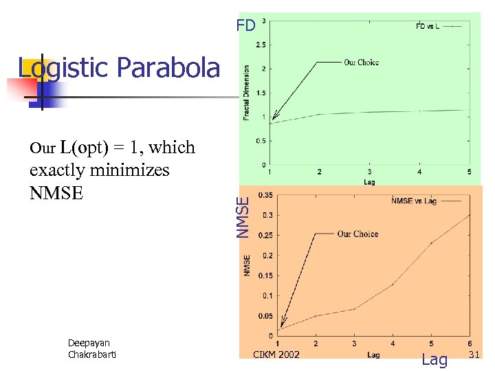FD Logistic Parabola exactly minimizes NMSE Deepayan Chakrabarti NMSE Our L(opt) = 1, which CIKM 2002 Lag 31

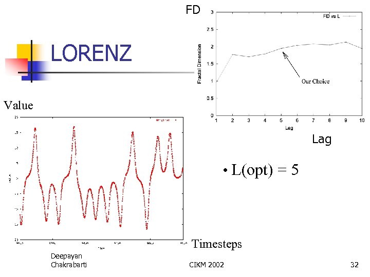FD LORENZ Value Lag • L(opt) = 5 Timesteps Deepayan Chakrabarti CIKM 2002 32

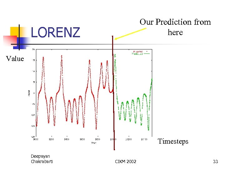Our Prediction from here LORENZ Value Timesteps Deepayan Chakrabarti CIKM 2002 33

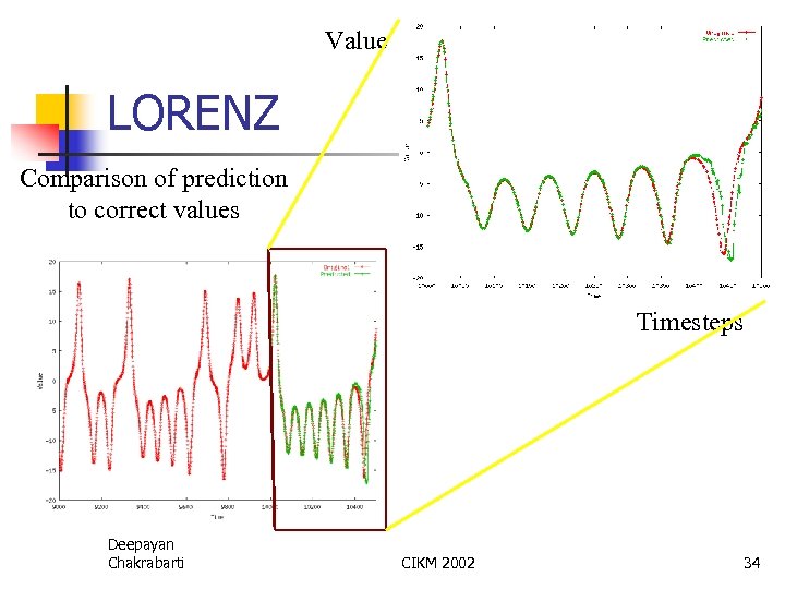Value LORENZ Comparison of prediction to correct values Timesteps Deepayan Chakrabarti CIKM 2002 34

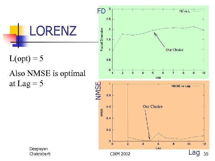FD LORENZ Also NMSE is optimal at Lag = 5 Deepayan Chakrabarti NMSE L(opt) = 5 CIKM 2002 Lag 35

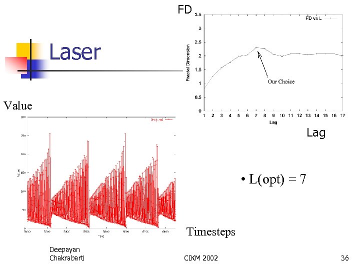FD Laser Value Lag • L(opt) = 7 Timesteps Deepayan Chakrabarti CIKM 2002 36

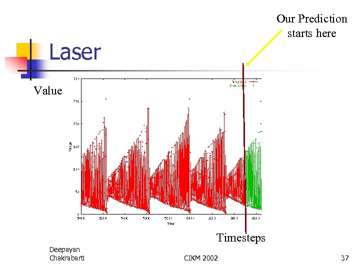Our Prediction starts here Laser Value Timesteps Deepayan Chakrabarti CIKM 2002 37

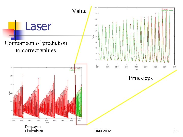Value Laser Comparison of prediction to correct values Timesteps Deepayan Chakrabarti CIKM 2002 38

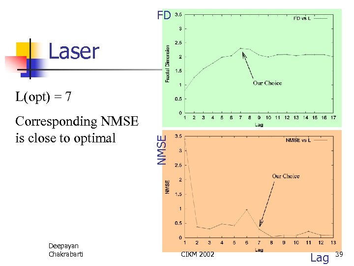FD Laser Corresponding NMSE is close to optimal Deepayan Chakrabarti NMSE L(opt) = 7 CIKM 2002 Lag 39

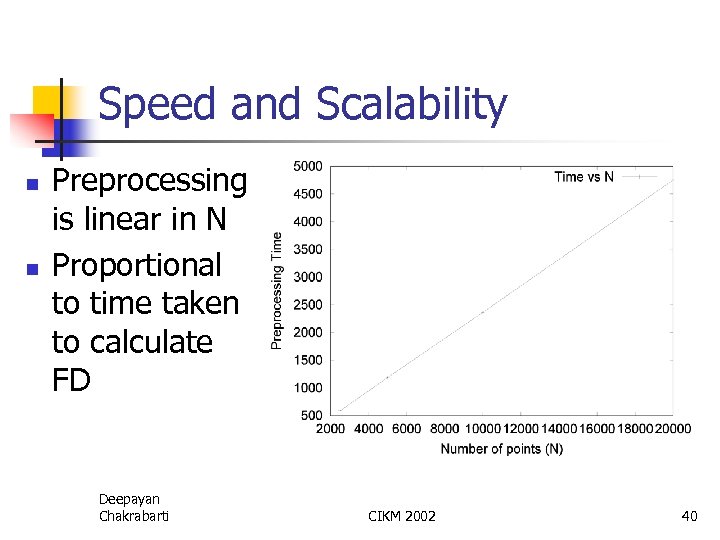Speed and Scalability n n Preprocessing is linear in N Proportional to time taken to calculate FD Deepayan Chakrabarti CIKM 2002 40

Outline n n Introduction/Motivation Survey and Lag Plots Exact Problem Formulation Proposed Method n n Fractal Dimensions Background Our method Results Conclusions Deepayan Chakrabarti CIKM 2002 41

Conclusions Our Method: ü Automatically set parameters ü ü ü L(opt) (answers Q 1) k(opt) (answers Q 2) In linear time on N Deepayan Chakrabarti CIKM 2002 42

Conclusions n n Black-box non-linear time series forecasting Fractal Dimensions give a fast, automated method to set all parameters So, given any time series, we can automatically build a prediction system Useful in a sensor network setting Deepayan Chakrabarti CIKM 2002 43

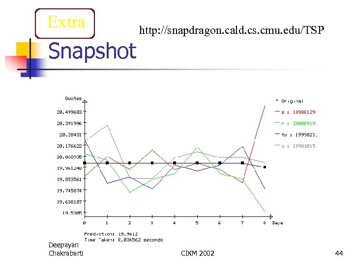Extra http: //snapdragon. cald. cs. cmu. edu/TSP Snapshot Deepayan Chakrabarti CIKM 2002 44

Extra Future Work n n Feature Selection Multi-sequence prediction Deepayan Chakrabarti CIKM 2002 45

Extra Discussion – Some other problems How to forecast? Given: • x 1, x 2, …, x. N • L(opt) • k(opt) How to find the k(opt) nearest neighbors quickly? Deepayan Chakrabarti CIKM 2002 46

Extra Motivation Forecasting also allows us to • Find outliers anything that doesn’t match our prediction! • Find patterns if different circumstances lead to similar predictions, they may be related. Deepayan Chakrabarti CIKM 2002 47

Motivation (Examples) Extra Traditional • EEGs : Patterns of electromagnetic impulses in the brain • Intensity variations of white dwarf stars • Highway usage over time Sensors • “Active Disks” forecasting / prefetching / buffering • “Smart House” sensors monitor situation in a house • Volcano monitoring Deepayan Chakrabarti CIKM 2002 48

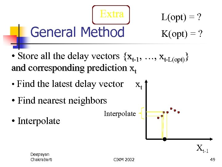Extra L(opt) = ? General Method K(opt) = ? • Store all the delay vectors {xt-1, …, xt-L(opt)} and corresponding prediction xt • Find the latest delay vector xt • Find nearest neighbors • Interpolate Deepayan Chakrabarti Interpolate Xt-1 CIKM 2002 49

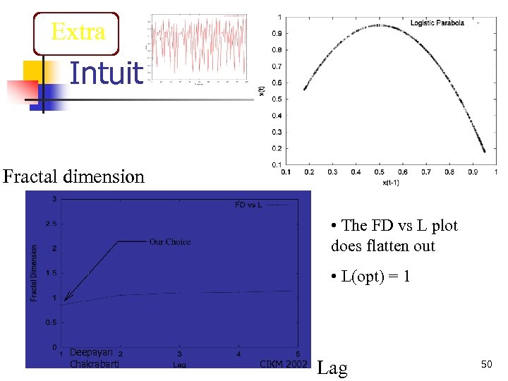Extra Intuition Fractal dimension • The FD vs L plot does flatten out • L(opt) = 1 Deepayan Chakrabarti CIKM 2002 Lag 50

Extra Inside Theory n n n Internal state may be unobserved But the delay vector space is a faithful reconstruction of the internal system state So prediction in delay vector space is as good as prediction in state space Deepayan Chakrabarti CIKM 2002 51

Fractal Dimensions n n Extra Many real-world datasets have fractional intrinsic dimension There exist fast (O(N)) methods to calculate the fractal dimension of a cloud of points [Belussi/1995] Deepayan Chakrabarti CIKM 2002 52

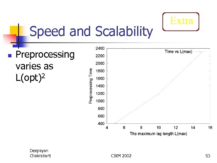Speed and Scalability n Extra Preprocessing varies as L(opt)2 Deepayan Chakrabarti CIKM 2002 53