Extending the multilevel model for change ALDA Chapter

Extending the multilevel model for change ALDA, Chapter Five “Change is a measure of time” Edwin Way Teale John B. Willett & Judith D. Singer Harvard Graduate School of Education

Chapter 5: Treating TIME more flexibly General idea: Although all our examples have been equally spaced, time-structured, and fully balanced, the multilevel model for change is actually far more flexible Variably spaced measurement occasions (§ 5. 1)—each individual can have his or her own customized data collection schedule Varying numbers of waves of data (§ 5. 2)—not everyone need have the same number of waves of data Allows us to handle missing data Can even include individuals with just one or two waves Including time-varying predictors (§ 5. 3) The values of some predictors vary over time They’re easy to include and can have powerful interpretations Re-centering the effect of TIME (§ 5. 4) Initial status is not the only centering constant for TIME Recentering TIME in the level-1 model improves interpretation in the level-2 model © Singer & Willett, page 2

Example for handling variably spaced waves: Reading achievement over time Data source: Children of the National Longitudinal Survey of Youth (CNLSY) Sample: 89 children Each approximately 6 years old at study start Research design 3 waves of data collected in 1986, 1988, and 1990, when the children were to be “in their 6 th yr, ” “in their 8 th yr, ” and “in their 10 th yr” Of course, not each child was tested on his/her birthday or half-birthday, which creates the variably spaced waves The outcome, PIAT, is the child’s unstandardized score on the reading portion of the Peabody Individual Achievement Test – Not standardized for age so we can see growth over time No substantive predictors to keep the example simple Research question How do PIAT scores change over time? © Singer & Willett, page 3

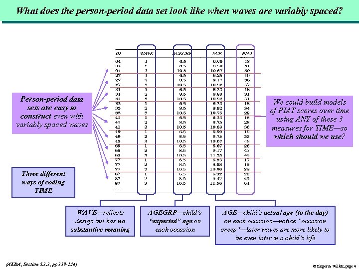What does the person-period data set look like when waves are variably spaced? Person-period data sets are easy to construct even with variably spaced waves We could build models of PIAT scores over time using ANY of these 3 measures for TIME—so which should we use? Three different ways of coding TIME WAVE—reflects design but has no substantive meaning (ALDA, Section 5. 1. 1, pp 139 -144) AGEGRP—child’s “expected” age on each occasion AGE—child’s actual age (to the day) on each occasion—notice “occasion creep”—later waves are more likely to be even later in a child’s life © Singer & Willett, page 4

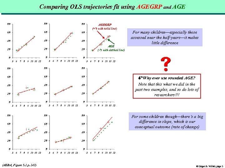Comparing OLS trajectories fit using AGEGRP and AGEGRP (+’s with solid line) AGE ( • ’s with dashed line) For many children—especially those assessed near the half-years—it makes little difference Why ever use rounded AGE? Note that this what we did in the past two examples, and so do lots of researchers!!! For some children though—there’s a big difference in slope, which is our conceptual outcome (rate of change) (ALDA, Figure 5. 1 p. 143) © Singer & Willett, page 5

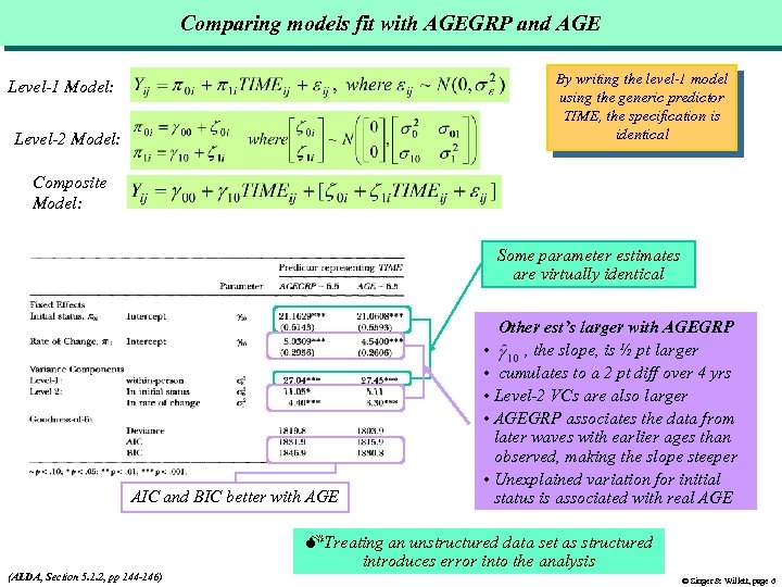Comparing models fit with AGEGRP and AGE By writing the level-1 model using the generic predictor TIME, the specification is identical Level-1 Model: Level-2 Model: Composite Model: Some parameter estimates are virtually identical AIC and BIC better with AGE Other est’s larger with AGEGRP • , the slope, is ½ pt larger • cumulates to a 2 pt diff over 4 yrs • Level-2 VCs are also larger • AGEGRP associates the data from later waves with earlier ages than observed, making the slope steeper • Unexplained variation for initial status is associated with real AGE Treating an unstructured data set as structured introduces error into the analysis (ALDA, Section 5. 1. 2, pp 144 -146) © Singer & Willett, page 6

Example for handling varying numbers of waves: Wages of HS dropouts Data source: Murnane, Boudett and Willett (1999), Evaluation Review Sample: 888 male high school dropouts Based on the National Longitudinal Survey of Youth (NLSY) Tracked from first job since HS dropout, when the men varied in age from 14 to 17 Research design Each interviewed between 1 and 13 times Interviews were approximately annual, but some were every 2 years Each wave’s interview conducted at different times during the year Both variable number and spacing of waves Outcome is log(WAGES), inflation adjusted natural logarithm of hourly wage Research question How do log(WAGES) change over time? Do the wage trajectories differ by ethnicity and highest grade completed? © Singer & Willett, page 7

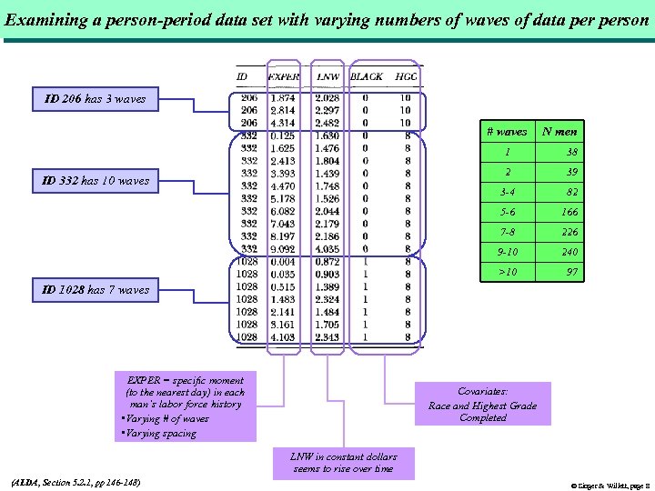Examining a person-period data set with varying numbers of waves of data person ID 206 has 3 waves # waves N men 1 2 39 3 -4 82 5 -6 166 7 -8 226 9 -10 240 >10 ID 332 has 10 waves 38 97 ID 1028 has 7 waves EXPER = specific moment (to the nearest day) in each man’s labor force history • Varying # of waves • Varying spacing Covariates: Race and Highest Grade Completed LNW in constant dollars seems to rise over time (ALDA, Section 5. 2. 1, pp 146 -148) © Singer & Willett, page 8

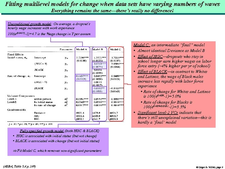Fitting multilevel models for change when data sets have varying numbers of waves Everything remains the same—there’s really no difference! Unconditional growth model: On average, a dropout’s hourly wage increases with work experience 100(e(0. 0457)-1)=4. 7 is the %age change in Y per annum Model C: an intermediate “final” model • Almost identical Deviance as Model B • Effect of HGC—dropouts who stay in school longer earn higher wages on labor force entry (~4% higher per yr of school) • Effect of BLACK—in contrast to Whites and Latinos, the wage of Black males increase less rapidly with labor force experience • Rate of change for Whites and Latinos is 100(e 0. 489 -1)=5. 0% • Rate of change for Blacks is 100(e 0. 489 -0. 0161 -1)=3. 3% • Significant level-2 VCs indicate that there’s still unexplained variation—this is hardly a ‘final’ model Fully specified growth model (both HGC & BLACK) • HGC is associated with initial status (but not change) • BLACK is associated with change (but not initial status) Fit Model C, which removes non-significant parameters (ALDA, Table 5. 4 p. 149) © Singer & Willett, page 9

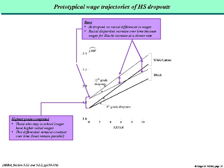Prototypical wage trajectories of HS dropouts Race • At dropout, no racial differences in wages • Racial disparities increase over time because wages for Blacks increase at a slower rate Highest grade completed • Those who stay in school longer have higher initial wages • This differential remains constant over time (lines remain parallel) (ALDA, Section 5. 2. 1 and 5. 2. 2, pp 150 -156) © Singer & Willett, page 10

Practical advice: Problems can arise when analyzing unbalanced data sets The multilevel model for change is designed to handle unbalanced data sets, and in most circumstances, it does its job well, however… When imbalance is severe, or lots of people have just 1 or 2 waves of data, problems can occur You may not estimate some parameters (well) Iterative fitting algorithms may not converge Some estimates may hit boundary constraints Problem is usually manifested via VCs not fixed effects (because the fixed portion of the model is like a ‘regular regression model”). Software packages may not issue clear warning signs If you’re lucky, you’ll get negative variance components Another sign is too much time to convergence (or no convergence) Most common problem: your model is overspecified Most common solution: simplify the model Many practical strategies discussed in ALDA, Section 5. 2. 2 Another major advantage of the multilevel model for change: How easy it is to include time-varying predictors (ALDA, Section 5. 2. 2, pp 151 -156) © Singer & Willett, page 11

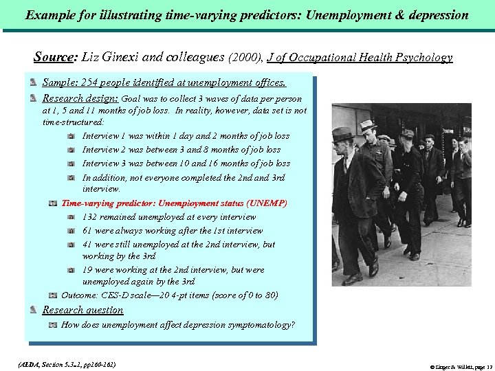Example for illustrating time-varying predictors: Unemployment & depression Source: Liz Ginexi and colleagues (2000), J of Occupational Health Psychology Sample: 254 people identified at unemployment offices. Research design: Goal was to collect 3 waves of data person at 1, 5 and 11 months of job loss. In reality, however, data set is not time-structured: Interview 1 was within 1 day and 2 months of job loss Interview 2 was between 3 and 8 months of job loss Interview 3 was between 10 and 16 months of job loss In addition, not everyone completed the 2 nd and 3 rd interview. Time-varying predictor: Unemployment status (UNEMP) 132 remained unemployed at every interview 61 were always working after the 1 st interview 41 were still unemployed at the 2 nd interview, but working by the 3 rd 19 were working at the 2 nd interview, but were unemployed again by the 3 rd Outcome: CES-D scale— 20 4 -pt items (score of 0 to 80) Research question How does unemployment affect depression symptomatology? (ALDA, Section 5. 3. . 1, pp 160 -161) © Singer & Willett, page 12

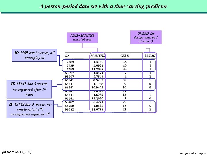A person-period data set with a time-varying predictor TIME=MONTHS since job loss UNEMP (by design, must be 1 at wave 1) ID 7589 has 3 waves, all unemployed ID 65641 has 3 waves, re-employed after 1 st wave ID 53782 has 3 waves, reemployed at 2 nd, unemployed again at 3 rd (ALDA, Table 5. 6, p 161) © Singer & Willett, page 13

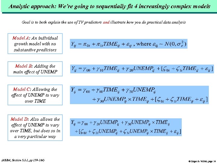Analytic approach: We’re going to sequentially fit 4 increasingly complex models Goal is to both explain the use of TV predictors and illustrate how you do practical data analysis Model A: An individual growth model with no substantive predictors Model B: Adding the main effect of UNEMP Model C: Allowing the effect of UNEMP to vary over TIME Model D: Also allows the effect of UNEMP to vary over TIME, but does so in a very particular way (ALDA, Section 5. 3. 1, pp 159 -164) © Singer & Willett, page 14

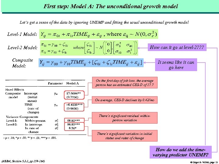First step: Model A: The unconditional growth model Let’s get a sense of the data by ignoring UNEMP and fitting the usual unconditional growth model Level-1 Model: Level-2 Model: How can it go at level-2? ? ? Composite Model: It seems like it can go here On the first day of job loss, the average person has an estimated CES-D of 17. 7 On average, CES-D declines by 0. 42/mo There’s significant residual withinperson variation There’s significant variation in initial status and rates of change How do we add the timevarying predictor UNEMP? (ALDA, Section 5. 3. 1, pp 159 -164) © Singer & Willett, page 15

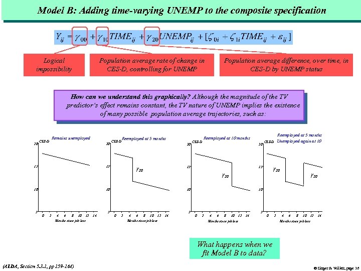Model B: Adding time-varying UNEMP to the composite specification Logical impossibility Population average rate of change in CES-D, controlling for UNEMP Population average difference, over time, in CES-D by UNEMP status How can we understand this graphically? Although the magnitude of the TV predictor’s effect remains constant, the TV nature of UNEMP implies the existence of many possible population average trajectories, such as: 20 Remains unemployed CES-D 20 15 20 g 20 15 0 2 4 6 8 10 12 Months since job loss 14 5 CES-D Reemployed at 10 months 20 15 0 2 4 6 g 20 15 10 8 10 Months since job loss 12 14 5 Reemployed at 5 months Unemployed again at 10 CES-D g 20 10 10 5 CES-D Reemployed at 5 months g 20 10 0 2 4 6 8 10 12 14 5 0 Months since job loss 2 4 6 8 10 12 14 Months since job loss What happens when we fit Model B to data? (ALDA, Section 5. 3. 1, pp 159 -164) © Singer & Willett, page 16

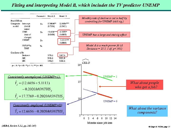Fitting and interpreting Model B, which includes the TV predictor UNEMP Monthly rate of decline is cut in half by controlling for UNEMP (still sig. ) UNEMP has a large and stat sig effect Model A is a much poorer fit ( Deviance = 25. 5, 1 df, p<. 001) 20 CES-D Consistently unemployed (UNEMP=1): UNEMP = 1 15 What about people who get a job? 10 UNEMP = 0 Consistently employed (UNEMP=0): 5 What about the variance components? 0 2 4 6 8 10 12 14 Months since job loss (ALDA, Section 5. 3. 1, pp. 162 -167) © Singer & Willett, page 17

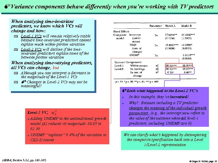Variance components behave differently when you’re working with TV predictors When analyzing time-invariant predictors, we know which VCs will change and how: Level-1 VCs will remain relatively stable because time-invariant predictors cannot explain much within-person variation Level-2 VCs will decline if the timeinvariant predictors explain some of the between person variation When analyzing time-varying predictors, all VCs can change, but Although you can interpret a decrease in the magnitude of the Level-1 VCs Changes in Level-2 VCs may not be meaningful! Level-1 VC, Adding UNEMP to the unconditional growth model (A) reduces its magnitude 68. 85 to 62. 39 UNEMP “explains” 9. 4% of the variation in CES-D scores (ALDA, Section 5. 3. 1, pp. 162 -167) Look what happened to the Level-2 VC’s In this example, they’ve increased! Why? : Because including a TV predictor changes the meaning of the individual growth parameters (e. g. , the intercept now refers to the value of the outcome when all level-1 predictors, including UNEMP are 0). We can clarify what’s happened by decomposing the composite specification back into a Level 1/Level-2 representation © Singer & Willett, page 18

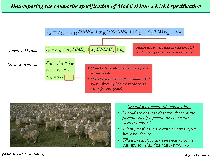Decomposing the composite specification of Model B into a L 1/L 2 specification Level-1 Model: Level-2 Models: Unlike time-invariant predictors, TV predictors go into the level-1 model • Model B’s level-2 model for 2 i has no residual! • Model B automatically assumes that 2 i is “fixed” (that it has the same value for everyone). Should we accept this constraint? • Should we assume that the effect of the person-specific predictor is constant across people? • When predictors are time-invariant, we have no choice • When predictors are time-varying, we can try to relax this assumption (ALDA, Section 5. 3. 1, pp. 168 -169) © Singer & Willett, page 19

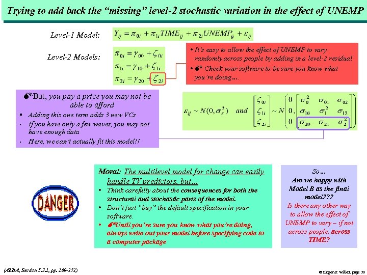Trying to add back the “missing” level-2 stochastic variation in the effect of UNEMP Level-1 Model: Level-2 Models: • It’s easy to allow the effect of UNEMP to vary randomly across people by adding in a level-2 residual • Check your software to be sure you know what you’re doing…. But, you pay a price you may not be able to afford § Adding this one term adds 3 new VCs § If you have only a few waves, you may not have enough data § Here, we can’t actually fit this model!! Moral: The multilevel model for change can easily handle TV predictors, but… • Think carefully about the consequences for both the structural and stochastic parts of the model. • Don’t just “buy” the default specification in your software. • Until you’re sure you know what you’re doing, always write out your model before specifying code to a computer package (ALDA, Section 5. 3. 1, pp. 169 -171) So… Are we happy with Model B as the final model? ? ? Is there any other way to allow the effect of UNEMP to vary – if not across people, across TIME? © Singer & Willett, page 20

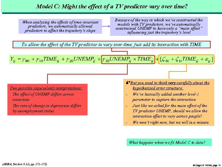Model C: Might the effect of a TV predictor vary over time? When analyzing the effects of time-invariant predictors, we automatically allowed predictors to affect the trajectory’s slope Because of the way in which we’ve constructed the models with TV predictors, we’ve automatically constrained UNEMP to have only a “main effect” influencing just the trajectory’s level To allow the effect of the TV predictor to vary over time, just add its interaction with TIME Two possible (equivalent) interpretations: The effect of UNEMP differs across occasions The rate of change in depression differs by unemployment status But you need to think very carefully about the hypothesized error structure: We’ve basically added another level-1 parameter to capture the interaction Just like we asked for the main effect of the TV predictor UNEMP, should we allow the interaction effect to vary across people? We won’t right now, but we will in a minute. What happens when we fit Model C to data? (ALDA, Section 5. 3. 2, pp. 171 -172) © Singer & Willett, page 21

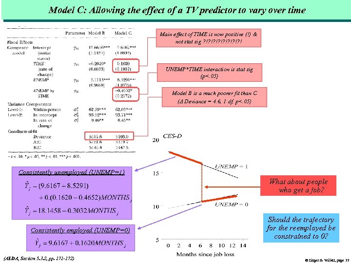Model C: Allowing the effect of a TV predictor to vary over time Main effect of TIME is now positive (!) & not stat sig ? !? !? !? ! UNEMP*TIME interaction is stat sig (p<. 05) Model B is a much poorer fit than C ( Deviance = 4. 6, 1 df, p<. 05) Consistently unemployed (UNEMP=1) What about people who get a job? Consistently employed (UNEMP=0) (ALDA, Section 5. 3. 2, pp. 171 -172) Should the trajectory for the reemployed be constrained to 0? © Singer & Willett, page 22

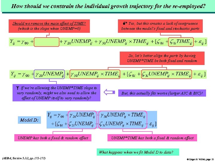How should we constrain the individual growth trajectory for the re-employed? Should we remove the main effect of TIME? (which is the slope when UNEMP=0) Yes, but this creates a lack of congruence between the model’s fixed and stochastic parts So, let’s better align the parts by having UNEMP*TIME be both fixed and random If we’re allowing the UNEMP*TIME slope to vary randomly, might we also need to allow the effect of UNEMP itself to vary randomly? But, this actually fits worse (larger AIC & BIC)! Model D: UNEMP has both a fixed & random effect UNEMP*TIME has both a fixed & random effect What happens when we fit Model D to data? (ALDA, Section 5. 3. 2, pp. 172 -173) © Singer & Willett, page 23

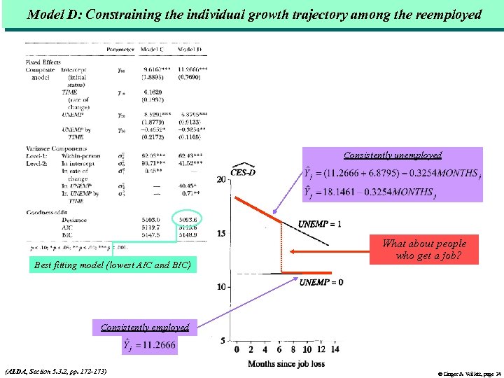Model D: Constraining the individual growth trajectory among the reemployed Consistently unemployed Best fitting model (lowest AIC and BIC) What about people who get a job? Consistently employed (ALDA, Section 5. 3. 2, pp. 172 -173) © Singer & Willett, page 24

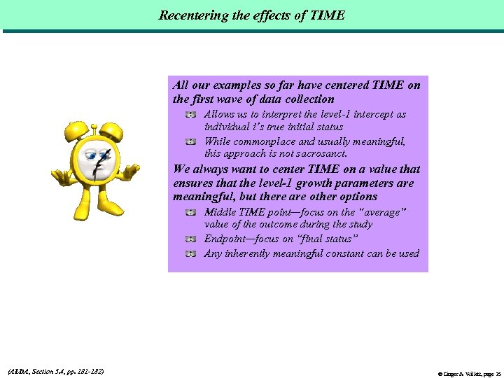Recentering the effects of TIME All our examples so far have centered TIME on the first wave of data collection Allows us to interpret the level-1 intercept as individual i’s true initial status While commonplace and usually meaningful, this approach is not sacrosanct. We always want to center TIME on a value that ensures that the level-1 growth parameters are meaningful, but there are other options Middle TIME point—focus on the “average” value of the outcome during the study Endpoint—focus on “final status” Any inherently meaningful constant can be used (ALDA, Section 5. 4, pp. 181 -182) © Singer & Willett, page 25

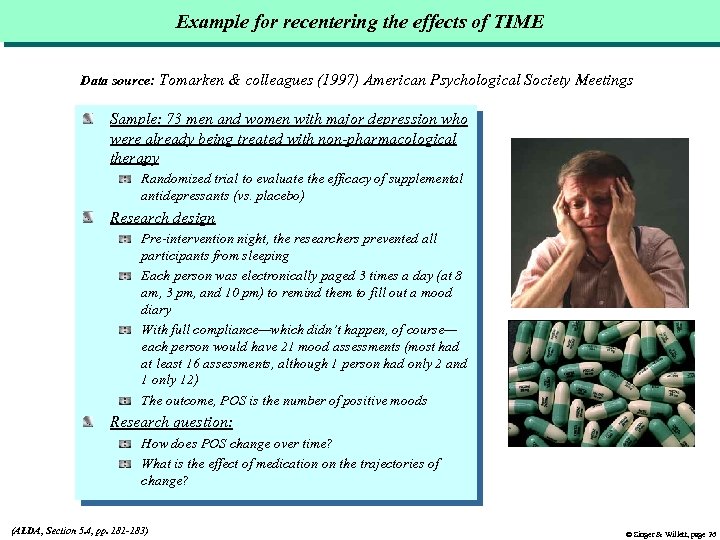Example for recentering the effects of TIME Data source: Tomarken & colleagues (1997) American Psychological Society Meetings Sample: 73 men and women with major depression who were already being treated with non-pharmacological therapy Randomized trial to evaluate the efficacy of supplemental antidepressants (vs. placebo) Research design Pre-intervention night, the researchers prevented all participants from sleeping Each person was electronically paged 3 times a day (at 8 am, 3 pm, and 10 pm) to remind them to fill out a mood diary With full compliance—which didn’t happen, of course— each person would have 21 mood assessments (most had at least 16 assessments, although 1 person had only 2 and 1 only 12) The outcome, POS is the number of positive moods Research question: How does POS change over time? What is the effect of medication on the trajectories of change? (ALDA, Section 5. 4, pp. 181 -183) © Singer & Willett, page 26

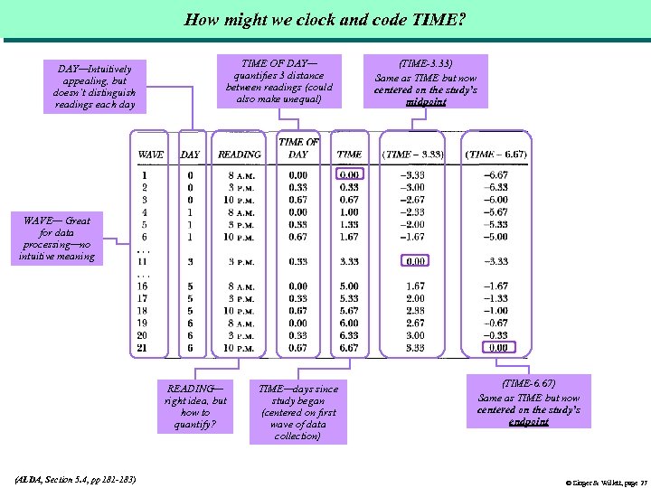How might we clock and code TIME? DAY—Intuitively appealing, but doesn’t distinguish readings each day TIME OF DAY— quantifies 3 distance between readings (could also make unequal) (TIME-3. 33) Same as TIME but now centered on the study’s midpoint WAVE— Great for data processing—no intuitive meaning READING— right idea, but how to quantify? (ALDA, Section 5. 4, pp 181 -183) TIME—days since study began (centered on first wave of data collection) (TIME-6. 67) Same as TIME but now centered on the study’s endpoint © Singer & Willett, page 27

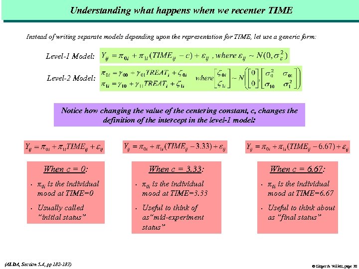Understanding what happens when we recenter TIME Instead of writing separate models depending upon the representation for TIME, let use a generic form: Level-1 Model: Level-2 Model: Notice how changing the value of the centering constant, c, changes the definition of the intercept in the level-1 model: When c = 0: • • π0 i is the individual mood at TIME=0 Usually called “initial status” (ALDA, Section 5. 4, pp 182 -183) When c = 3. 33: • • π0 i is the individual mood at TIME=3. 33 Useful to think of as“mid-experiment status” When c = 6. 67: • • π0 i is the individual mood at TIME=6. 67 Useful to think about as “final status” © Singer & Willett, page 28

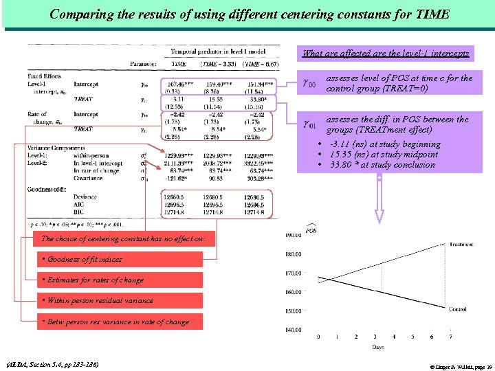Comparing the results of using different centering constants for TIME What are affected are the level-1 intercepts assesses level of POS at time c for the control group (TREAT=0) assesses the diff. in POS between the groups (TREATment effect) • -3. 11 (ns) at study beginning • 15. 35 (ns) at study midpoint • 33. 80 * at study conclusion The choice of centering constant has no effect on: • Goodness of fit indices • Estimates for rates of change • Within person residual variance • Betw person res variance in rate of change (ALDA, Section 5. 4, pp 183 -186) © Singer & Willett, page 29

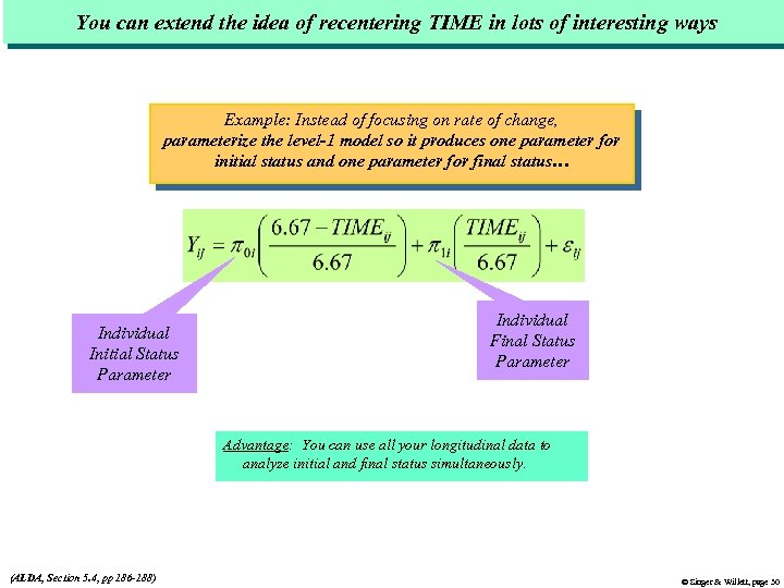You can extend the idea of recentering TIME in lots of interesting ways Example: Instead of focusing on rate of change, parameterize the level-1 model so it produces one parameter for initial status and one parameter for final status… Individual Initial Status Parameter Individual Final Status Parameter Advantage: You can use all your longitudinal data to analyze initial and final status simultaneously. (ALDA, Section 5. 4, pp 186 -188) © Singer & Willett, page 30