6f98645c601b9f98fadf33b210a67714.ppt
- Количество слайдов: 56
 Extended Learning Module D Decision Analysis with Spreadsheet Software © Mc. Graw-Hill Companies, Inc. , Mc. Graw-Hill/Irwin
 STUDENT LEARNING OUTCOMES 1. 2. 3. Define a list and list definition table within the context of spreadsheet software and describe the importance of each. Compare and contrast the Filter function and Custom Filter function in spreadsheet software. Describe the purpose of using conditional formatting. © Mc. Graw-Hill Companies, Inc. , Mc. Graw-Hill/Irwin
 STUDENT LEARNING OUTCOMES 4. 5. Define a pivot table and describe how you can use it to view summarized information by dimension. Describe the purpose of Goal Seek. © Mc. Graw-Hill Companies, Inc. , Mc. Graw-Hill/Irwin
 INTRODUCTION IT plays an important role in aiding decision making Spreadsheet tools can aid in decision making Filter Conditional formatting Pivot tables © Mc. Graw-Hill Companies, Inc. , Mc. Graw-Hill/Irwin
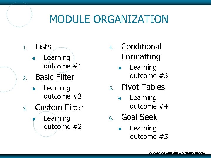 MODULE ORGANIZATION 1. Lists 2. Learning outcome #1 Learning outcome #2 5. Learning outcome #2 6. Learning outcome #3 Pivot Tables Custom Filter Conditional Formatting Basic Filter 3. 4. Learning outcome #4 Goal Seek Learning outcome #5 © Mc. Graw-Hill Companies, Inc. , Mc. Graw-Hill/Irwin
 LISTS List – information arranged in columns and rows Each column has one type of information First row contains headings or labels No blank rows Blank columns/rows all around © Mc. Graw-Hill Companies, Inc. , Mc. Graw-Hill/Irwin
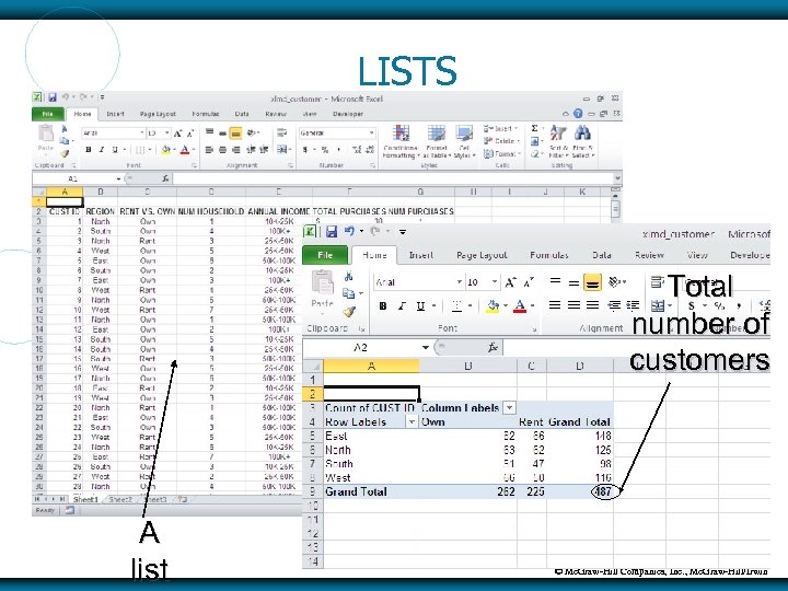 LISTS Total number of customers A list © Mc. Graw-Hill Companies, Inc. , Mc. Graw-Hill/Irwin
 List Definition Table List definition table – description of a list by column (see Figure D. 2 on pp. 388 -389) CUST ID – Unique ID for customer REGION – North, South, etc. RENT VS. OWN – customer rents or owns a home And so on © Mc. Graw-Hill Companies, Inc. , Mc. Graw-Hill/Irwin
 BASIC FILTER Filter function – filters a list and hides rows that don’t match criteria Good for seeing only certain rows of information Basic Filter supports only “equal to” criteria Example: customers in the North REGION © Mc. Graw-Hill Companies, Inc. , Mc. Graw-Hill/Irwin
 Basic Filter Steps 1. 2. 3. Open workbook (XLMD_Customer. xls from www. mhhe. com/haag) Click in any cell in the list Menu bar – click on Data and then click on Filter Will see list box arrows next to each label or column heading © Mc. Graw-Hill Companies, Inc. , Mc. Graw-Hill/Irwin
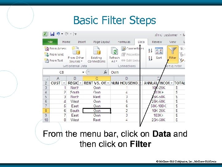 Basic Filter Steps From the menu bar, click on Data and then click on Filter © Mc. Graw-Hill Companies, Inc. , Mc. Graw-Hill/Irwin
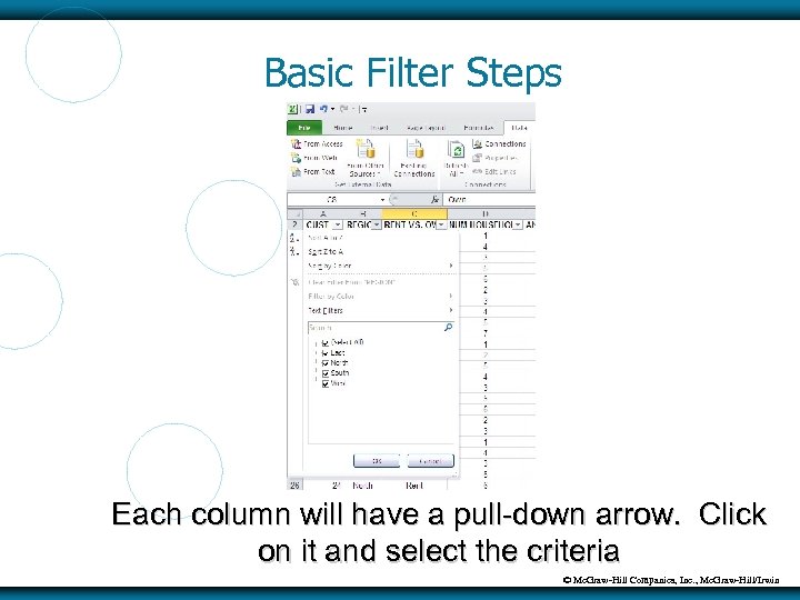 Basic Filter Steps Each column will have a pull-down arrow. Click on it and select the criteria © Mc. Graw-Hill Companies, Inc. , Mc. Graw-Hill/Irwin
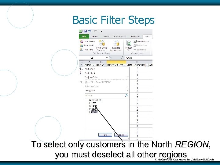 Basic Filter Steps To select only customers in the North REGION, you must deselect all other regions © Mc. Graw-Hill Companies, Inc. , Mc. Graw-Hill/Irwin
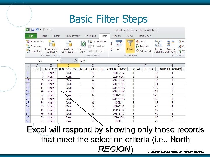 Basic Filter Steps Excel will respond by showing only those records that meet the selection criteria (i. e. , North REGION) © Mc. Graw-Hill Companies, Inc. , Mc. Graw-Hill/Irwin
 Turning off Basic Filter Perform either of the following From the menu bar, click on Data and then Filter Turn off selected column filtering by clicking on the appropriate list arrow box and clicking on Clear Filter from “columnname” where columnname is the name of the column © Mc. Graw-Hill Companies, Inc. , Mc. Graw-Hill/Irwin
 Basic Filter Can also filter on multiple columns Example Customers in North region (select North in REGION) Own a home (select Own in RENT VS. OWN) Only one household member (select 1 in NUM HOUSEHOLD) © Mc. Graw-Hill Companies, Inc. , Mc. Graw-Hill/Irwin
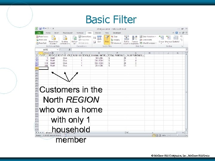 Basic Filter Customers in the North REGION who own a home with only 1 household member © Mc. Graw-Hill Companies, Inc. , Mc. Graw-Hill/Irwin
 CUSTOM FILTER Custom Filter function – hides all rows except those that meet criteria, besides “is equal to” Example Customers with more than 3 household members © Mc. Graw-Hill Companies, Inc. , Mc. Graw-Hill/Irwin
 Custom Filter Steps 1. 2. 3. 4. 5. Turn on Filter Click on pull-down arrow in appropriate column Click on Number Filters Complete Custom Auto. Filter dialog box with criteria Click on OK © Mc. Graw-Hill Companies, Inc. , Mc. Graw-Hill/Irwin
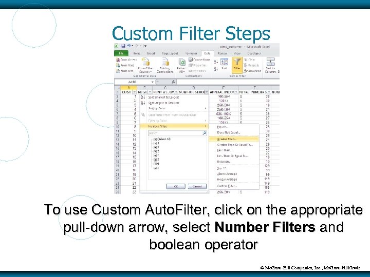 Custom Filter Steps To use Custom Auto. Filter, click on the appropriate pull-down arrow, select Number Filters and boolean operator © Mc. Graw-Hill Companies, Inc. , Mc. Graw-Hill/Irwin
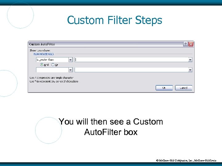 Custom Filter Steps You will then see a Custom Auto. Filter box © Mc. Graw-Hill Companies, Inc. , Mc. Graw-Hill/Irwin
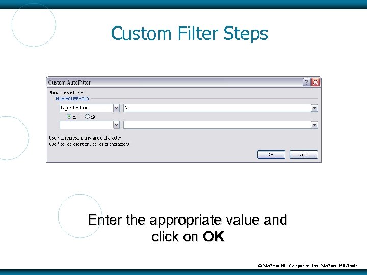 Custom Filter Steps Enter the appropriate value and click on OK © Mc. Graw-Hill Companies, Inc. , Mc. Graw-Hill/Irwin
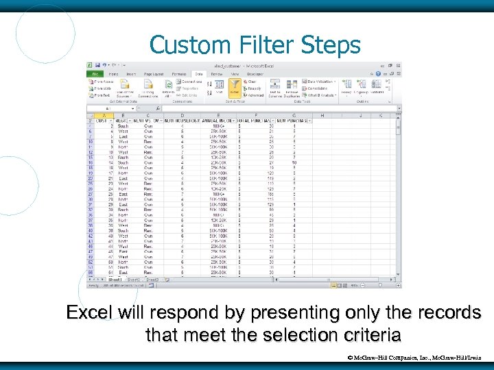 Custom Filter Steps Excel will respond by presenting only the records that meet the selection criteria © Mc. Graw-Hill Companies, Inc. , Mc. Graw-Hill/Irwin
 Another Custom Filter Example Customers who spent less than $20 or more than $100 © Mc. Graw-Hill Companies, Inc. , Mc. Graw-Hill/Irwin
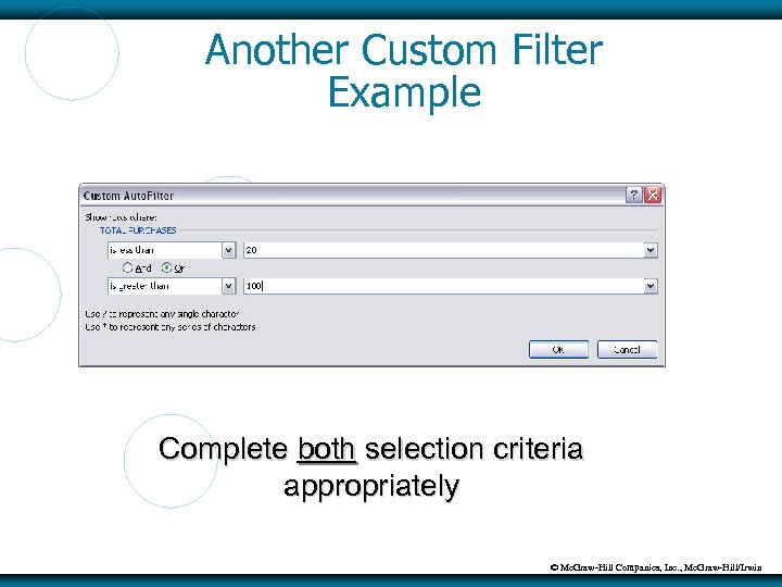 Another Custom Filter Example Complete both selection criteria appropriately © Mc. Graw-Hill Companies, Inc. , Mc. Graw-Hill/Irwin
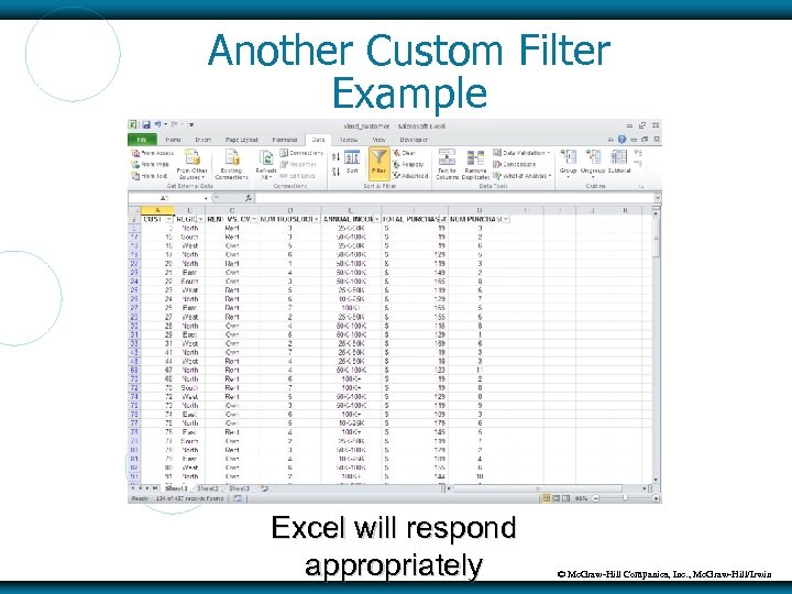 Another Custom Filter Example Excel will respond appropriately © Mc. Graw-Hill Companies, Inc. , Mc. Graw-Hill/Irwin
 CONDITIONAL FORMATTING Conditional formatting – highlights the information in a cell that meets some criteria Does not hide any rows Let’s you see the whole list While highlighting certain information Example Customers show purchased more than $100 © Mc. Graw-Hill Companies, Inc. , Mc. Graw-Hill/Irwin
 Conditional Formatting Steps 1. 2. 3. 4. 5. 6. Select entire appropriate column From menu bar, click on Home and then Conditional Formatting within Styles Select Highlight Cells Rules Click on the appropriate boolean operator Complete the dialog box Click on OK © Mc. Graw-Hill Companies, Inc. , Mc. Graw-Hill/Irwin
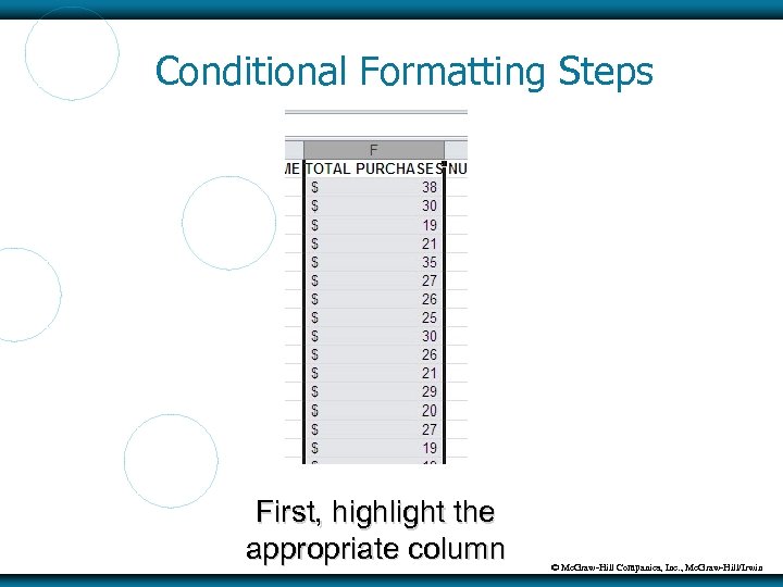 Conditional Formatting Steps First, highlight the appropriate column © Mc. Graw-Hill Companies, Inc. , Mc. Graw-Hill/Irwin
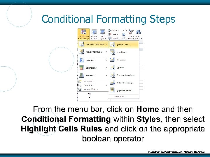 Conditional Formatting Steps From the menu bar, click on Home and then Conditional Formatting within Styles, then select Highlight Cells Rules and click on the appropriate boolean operator © Mc. Graw-Hill Companies, Inc. , Mc. Graw-Hill/Irwin
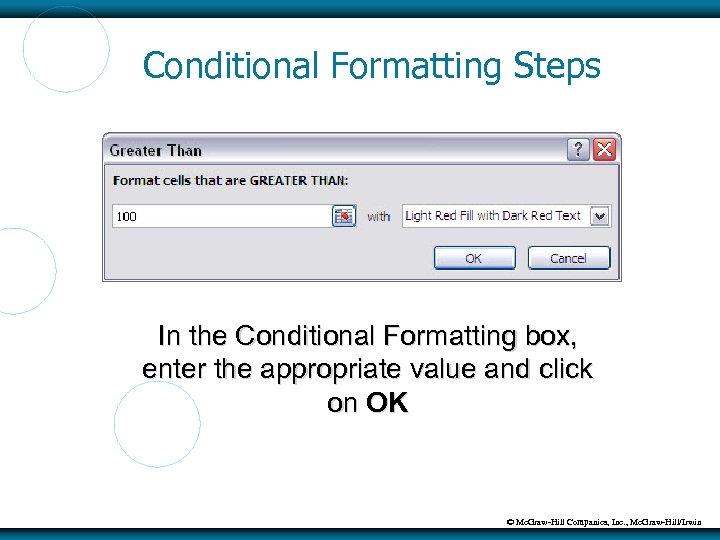 Conditional Formatting Steps In the Conditional Formatting box, enter the appropriate value and click on OK © Mc. Graw-Hill Companies, Inc. , Mc. Graw-Hill/Irwin
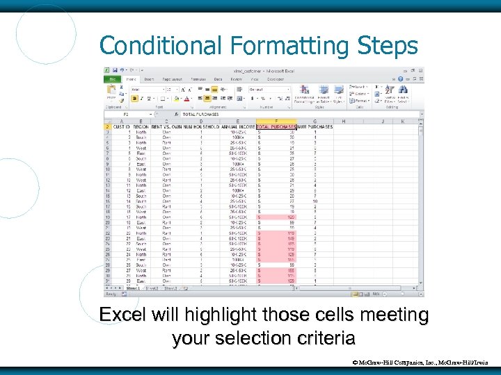 Conditional Formatting Steps Excel will highlight those cells meeting your selection criteria © Mc. Graw-Hill Companies, Inc. , Mc. Graw-Hill/Irwin
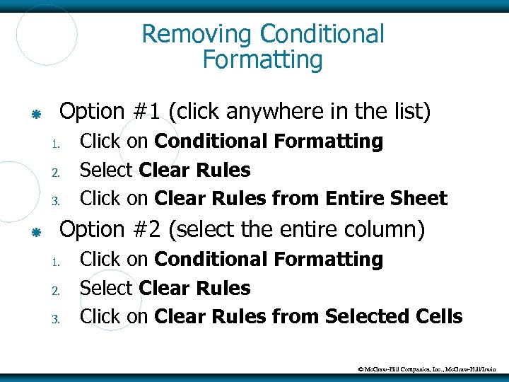 Removing Conditional Formatting Option #1 (click anywhere in the list) 1. 2. 3. Click on Conditional Formatting Select Clear Rules Click on Clear Rules from Entire Sheet Option #2 (select the entire column) 1. 2. 3. Click on Conditional Formatting Select Clear Rules Click on Clear Rules from Selected Cells © Mc. Graw-Hill Companies, Inc. , Mc. Graw-Hill/Irwin
 PIVOT TABLES Pivot table – enables you to group and summarize information Shows summaries of information by dimension Can be two-dimensional Can be three-dimensional Similar to data warehouse concept from Chapter 3 © Mc. Graw-Hill Companies, Inc. , Mc. Graw-Hill/Irwin
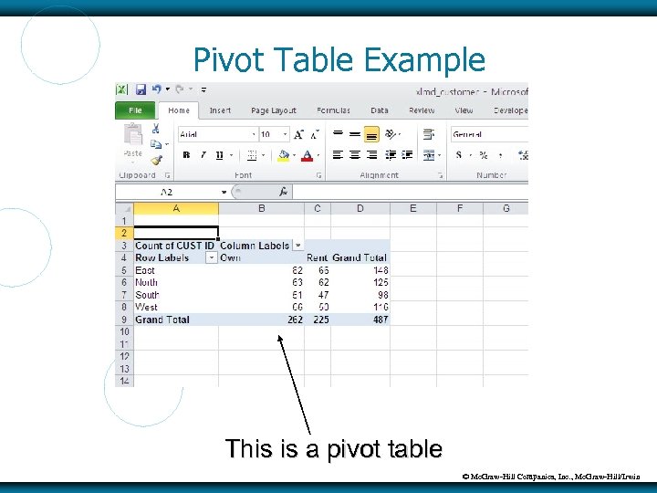 Pivot Table Example This is a pivot table © Mc. Graw-Hill Companies, Inc. , Mc. Graw-Hill/Irwin
 2 D Pivot Table Steps 1. 2. 3. 4. 5. Click anywhere in list From menu bar, click on Insert and then Pivot. Table Click on OK Drag/drop labels in row and column fields Provide appropriate formatting © Mc. Graw-Hill Companies, Inc. , Mc. Graw-Hill/Irwin
 2 D Pivot Table Count of customers By REGION By RENT VS. OWN © Mc. Graw-Hill Companies, Inc. , Mc. Graw-Hill/Irwin
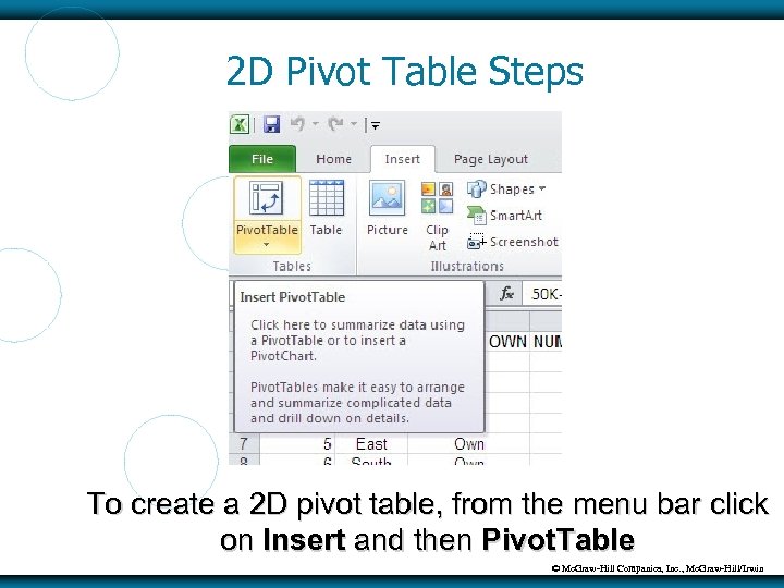 2 D Pivot Table Steps To create a 2 D pivot table, from the menu bar click on Insert and then Pivot. Table © Mc. Graw-Hill Companies, Inc. , Mc. Graw-Hill/Irwin
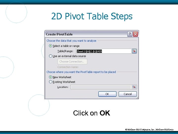 2 D Pivot Table Steps Click on OK © Mc. Graw-Hill Companies, Inc. , Mc. Graw-Hill/Irwin
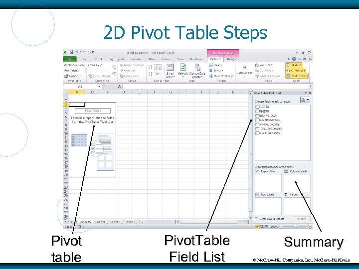 2 D Pivot Table Steps Pivot table Pivot. Table Field List Summary © Mc. Graw-Hill Companies, Inc. , Mc. Graw-Hill/Irwin
 2 D Pivot Table Steps Now, drag and drop appropriate column headings (labels) from the Pivot Table Field List Box to the appropriate places in the pivot table summary area Example: Number of customers by REGION RENT VS. OWN © Mc. Graw-Hill Companies, Inc. , Mc. Graw-Hill/Irwin
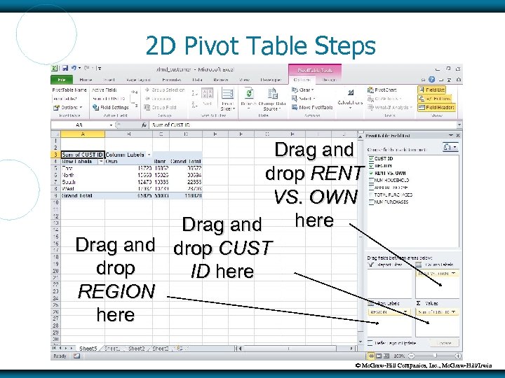 2 D Pivot Table Steps Drag and drop RENT VS. OWN here Drag and drop CUST drop ID here REGION here © Mc. Graw-Hill Companies, Inc. , Mc. Graw-Hill/Irwin
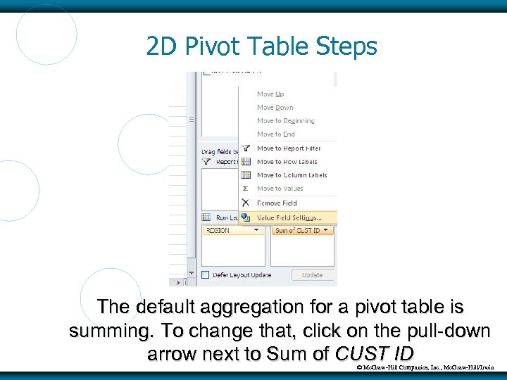 2 D Pivot Table Steps The default aggregation for a pivot table is summing. To change that, click on the pull-down arrow next to Sum of CUST ID © Mc. Graw-Hill Companies, Inc. , Mc. Graw-Hill/Irwin
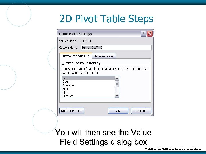 2 D Pivot Table Steps You will then see the Value Field Settings dialog box © Mc. Graw-Hill Companies, Inc. , Mc. Graw-Hill/Irwin
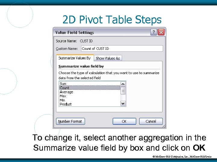 2 D Pivot Table Steps To change it, select another aggregation in the Summarize value field by box and click on OK © Mc. Graw-Hill Companies, Inc. , Mc. Graw-Hill/Irwin
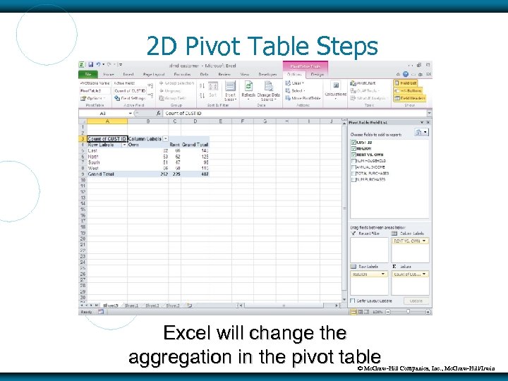 2 D Pivot Table Steps Excel will change the aggregation in the pivot table © Mc. Graw-Hill Companies, Inc. , Mc. Graw-Hill/Irwin
 Pivot Tables Can have multiple pieces of information in the body of the pivot table Example Count of customers (already present) Total of purchases (new information) Drag/drop TOTAL PURCHASES into Values in lower right portion of screen © Mc. Graw-Hill Companies, Inc. , Mc. Graw-Hill/Irwin
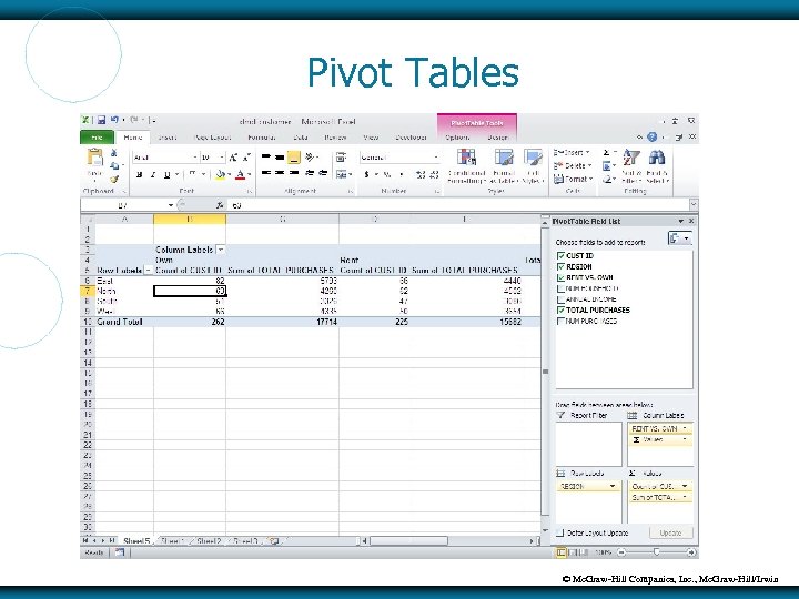 Pivot Tables © Mc. Graw-Hill Companies, Inc. , Mc. Graw-Hill/Irwin
 3 D Pivot Tables Desired dimensions REGION RENT VS. OWN NUM HOUSEHOLD Drag/drop NUM HOUSEHOLD into lower right portion of the screen called “Report Filter” © Mc. Graw-Hill Companies, Inc. , Mc. Graw-Hill/Irwin
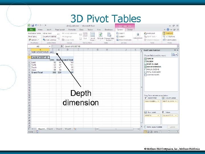 3 D Pivot Tables Depth dimension © Mc. Graw-Hill Companies, Inc. , Mc. Graw-Hill/Irwin
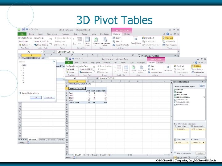 3 D Pivot Tables © Mc. Graw-Hill Companies, Inc. , Mc. Graw-Hill/Irwin
 GOAL SEEK Goal Seek works backward from objective to compute an unknown value Scenario (movie posters from Chapter 1): Buy poster for $4 and sell for $9 $2 shipping for each poster Fixed costs of $1, 500 per year What is the breakeven point? © Mc. Graw-Hill Companies, Inc. , Mc. Graw-Hill/Irwin
 GOAL SEEK – BREAKEVEN POINT Download XLMD_Break. Even. xls C 14 = C 13*C 7 C 15 = C 13*C 8 C 16 = C 13*C 9 C 18 = C 14 – C 15 – C 16 – C 17 Now, for a given net profit, we want Excel to compute Units Sold (C 13) © Mc. Graw-Hill Companies, Inc. , Mc. Graw-Hill/Irwin
 GOAL SEEK – BREAKEVEN POINT 1. 2. 3. 4. 5. 6. From menu bar, click on Data and What-If Analysis Select Goal Seek For Set cell, enter C 18 For To value, enter 30000 For By changing cell, enter C 13 Click on OK © Mc. Graw-Hill Companies, Inc. , Mc. Graw-Hill/Irwin
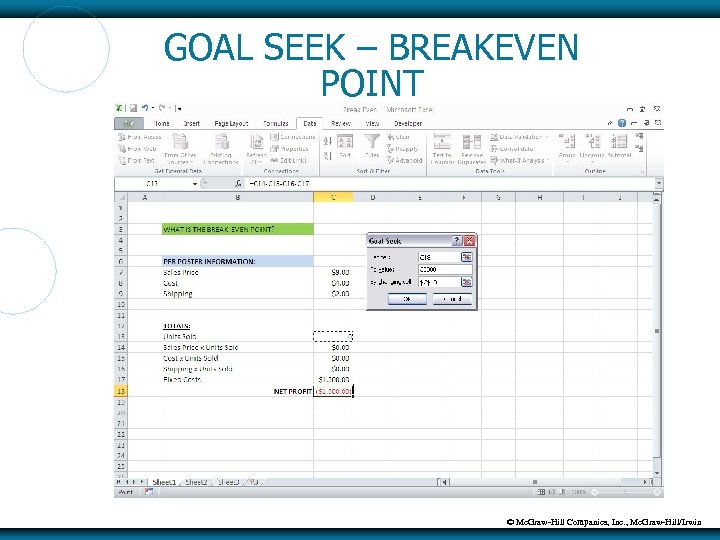 GOAL SEEK – BREAKEVEN POINT © Mc. Graw-Hill Companies, Inc. , Mc. Graw-Hill/Irwin
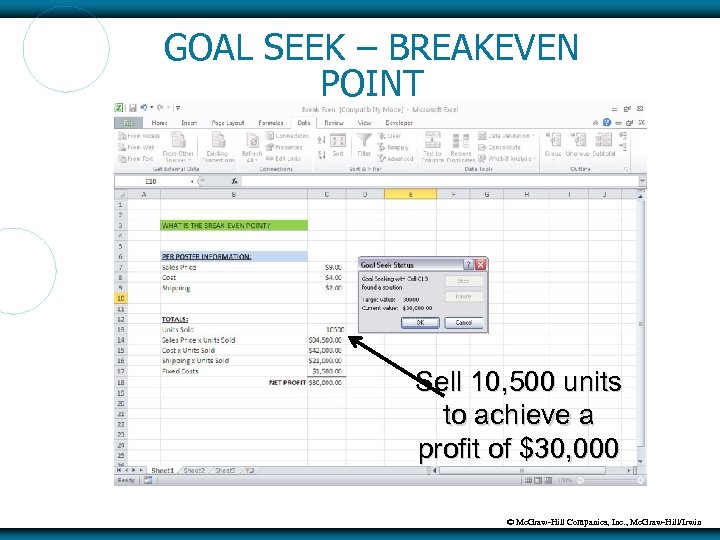 GOAL SEEK – BREAKEVEN POINT Sell 10, 500 units to achieve a profit of $30, 000 © Mc. Graw-Hill Companies, Inc. , Mc. Graw-Hill/Irwin


