a8e131e8e9ec58bb64c7949ae73f45d4.ppt
- Количество слайдов: 92
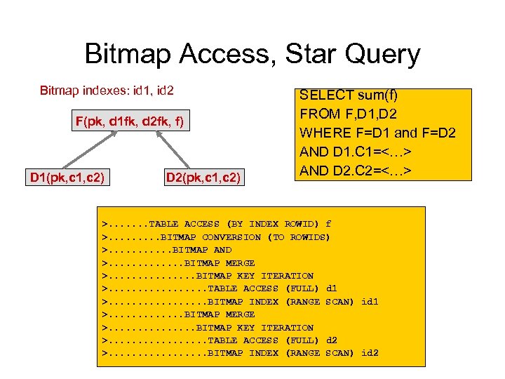
 Execution Oracle SQL Tuning An Introduction Toon Koppelaars Sr. IT Architect Central Bookhouse
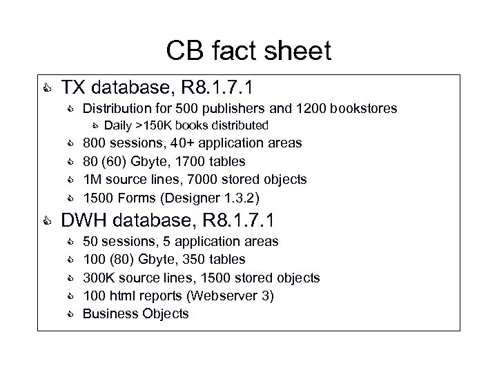 CB fact sheet C TX database, R 8. 1. 7. 1 C Distribution for 500 publishers and 1200 bookstores C C C Daily >150 K books distributed 800 sessions, 40+ application areas 80 (60) Gbyte, 1700 tables 1 M source lines, 7000 stored objects 1500 Forms (Designer 1. 3. 2) DWH database, R 8. 1. 7. 1 C C C 50 sessions, 5 application areas 100 (80) Gbyte, 350 tables 300 K source lines, 1500 stored objects 100 html reports (Webserver 3) Business Objects
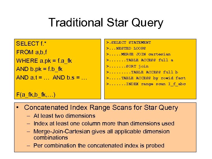
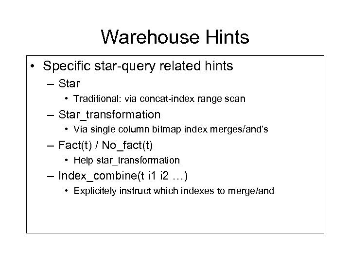
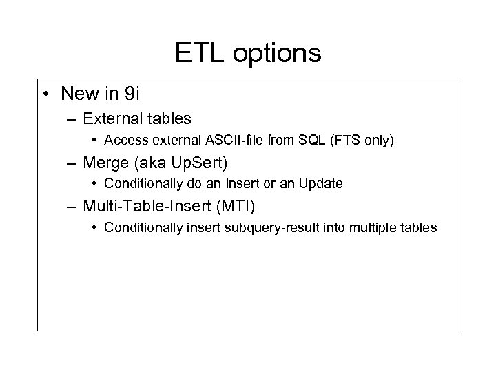
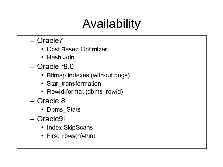
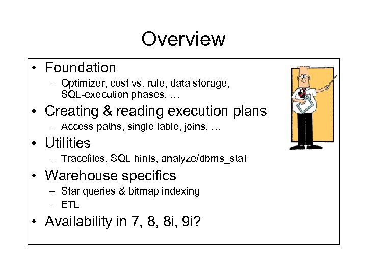 Overview • Foundation – Optimizer, cost vs. rule, data storage, SQL-execution phases, … • Creating & reading execution plans – Access paths, single table, joins, … • Utilities – Tracefiles, SQL hints, analyze/dbms_stat • Warehouse specifics – Star queries & bitmap indexing – ETL • Availability in 7, 8, 8 i, 9 i?
 Goals • Read execution plans • • Table access Index access Joins Subqueries • Understand execution plans • Understand performance • Basic understanding of SQL optimization • Start thinking how you should have executed it
 Next… • Basic Concepts (13) – Background information • SQL-Execution (50) – Read + understand
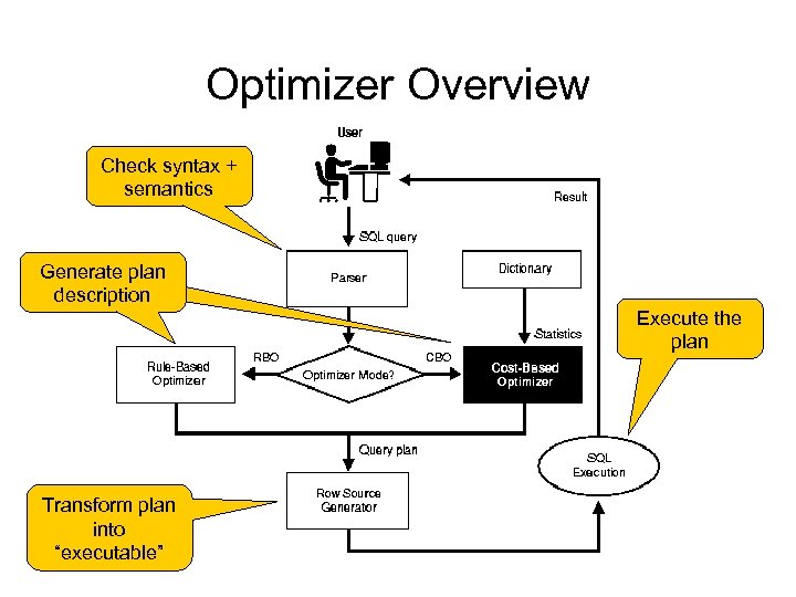 Optimizer Overview Check syntax + semantics Generate plan description Execute the plan Transform plan into “executable”
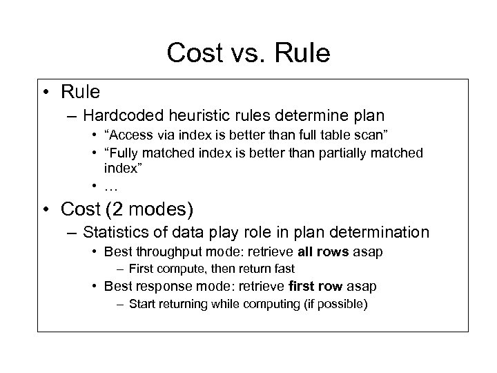 Cost vs. Rule • Rule – Hardcoded heuristic rules determine plan • “Access via index is better than full table scan” • “Fully matched index is better than partially matched index” • … • Cost (2 modes) – Statistics of data play role in plan determination • Best throughput mode: retrieve all rows asap – First compute, then return fast • Best response mode: retrieve first row asap – Start returning while computing (if possible)
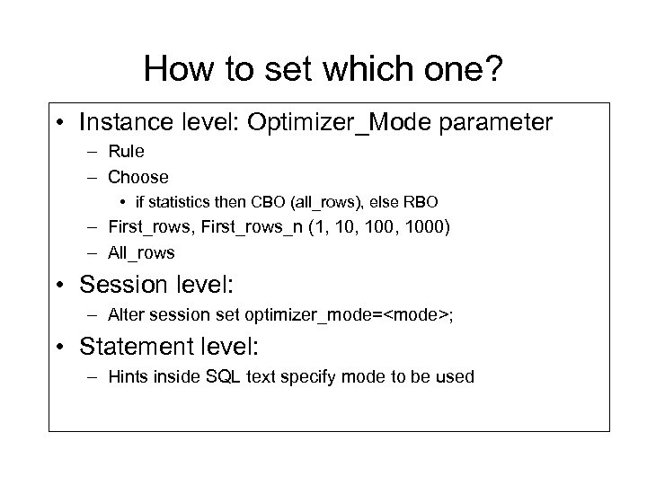 How to set which one? • Instance level: Optimizer_Mode parameter – Rule – Choose • if statistics then CBO (all_rows), else RBO – First_rows, First_rows_n (1, 100, 1000) – All_rows • Session level: – Alter session set optimizer_mode=
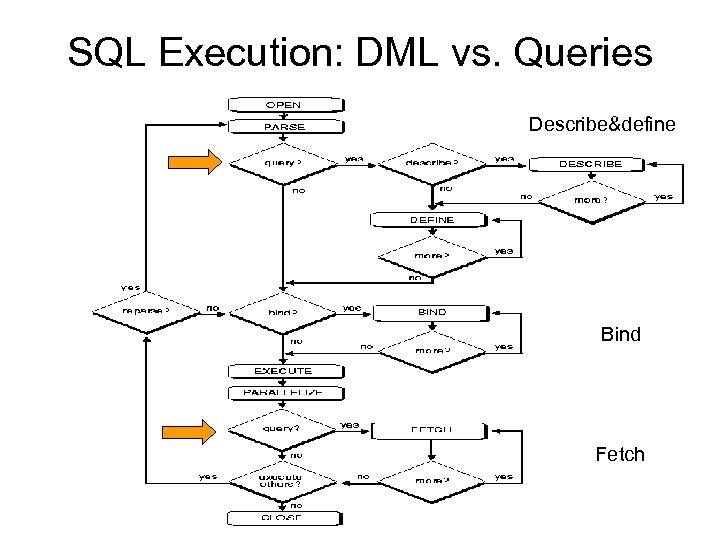 SQL Execution: DML vs. Queries Describe&define Bind Fetch
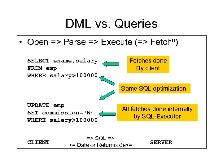 DML vs. Queries • Open => Parse => Execute (=> Fetchn) SELECT ename, salary FROM emp WHERE salary>100000 Fetches done By client Same SQL optimization UPDATE emp SET commission=‘N’ WHERE salary>100000 CLIENT All fetches done internally by SQL-Executor => SQL => <= Data or Returncode<= SERVER
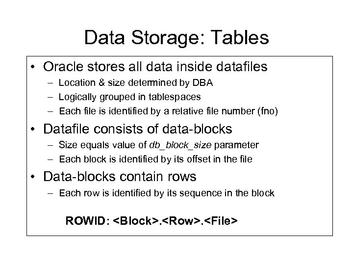 Data Storage: Tables • Oracle stores all data inside datafiles – Location & size determined by DBA – Logically grouped in tablespaces – Each file is identified by a relative file number (fno) • Datafile consists of data-blocks – Size equals value of db_block_size parameter – Each block is identified by its offset in the file • Data-blocks contain rows – Each row is identified by its sequence in the block ROWID:
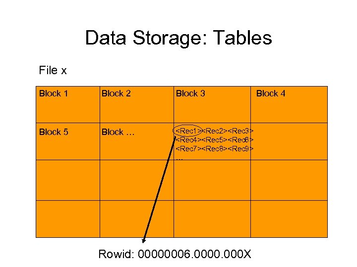 Data Storage: Tables File x Block 1 Block 2 Block 3 Block 5 Block …
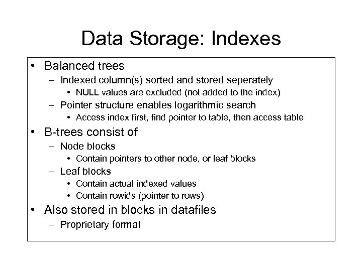 Data Storage: Indexes • Balanced trees – Indexed column(s) sorted and stored seperately • NULL values are excluded (not added to the index) – Pointer structure enables logarithmic search • Access index first, find pointer to table, then access table • B-trees consist of – Node blocks • Contain pointers to other node, or leaf blocks – Leaf blocks • Contain actual indexed values • Contain rowids (pointer to rows) • Also stored in blocks in datafiles – Proprietary format
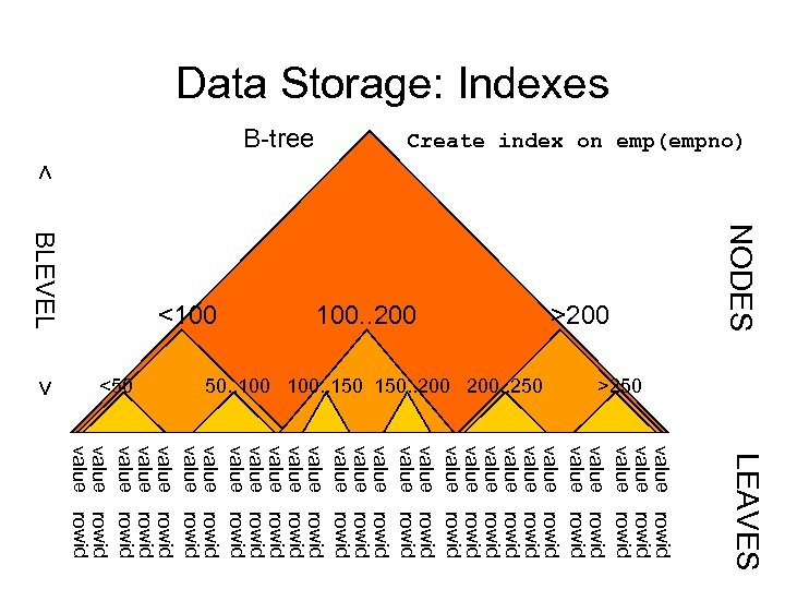 Data Storage: Indexes < NODES BLEVEL >250 50. . 100. . 150. . 200. . 250 > <50 >200 100. . 200 <100 Create index on emp(empno) B-tree rowid rowid rowid rowid rowid rowid rowid LEAVES value value value value value value value
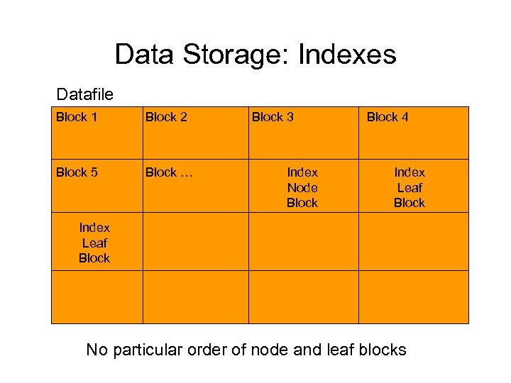 Data Storage: Indexes Datafile Block 1 Block 2 Block 5 Block … Block 3 Index Node Block 4 Index Leaf Block No particular order of node and leaf blocks
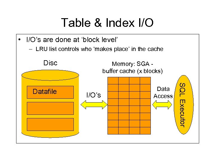 Table & Index I/O • I/O’s are done at ‘block level’ – LRU list controls who ‘makes place’ in the cache Disc I/O’s Data Access SQL Executor Datafile Memory: SGA buffer cache (x blocks)
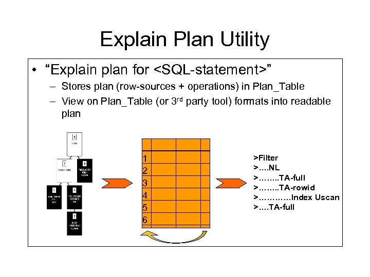 Explain Plan Utility • “Explain plan for
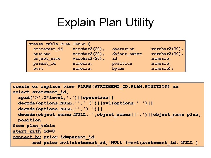 Explain Plan Utility create table PLAN_TABLE ( statement_id varchar 2(30), options varchar 2(30), object_name varchar 2(30), parent_id numeric, cost numeric, operation object_owner id position bytes varchar 2(30), numeric, numeric); create or replace view PLANS(STATEMENT_ID, PLAN, POSITION) as select statement_id, rpad('>', 2*level, '. ')||operation|| decode(options, NULL, '', ' (')||nvl(options, ' ')|| decode(options, NULL, '', ') ')|| decode(object_owner, NULL, '', object_owner||'. ')||object_name plan, position from plan_table start with id=0 connect by prior id=parent_id and prior nvl(statement_id, 'NULL')=nvl(statement_id, 'NULL')
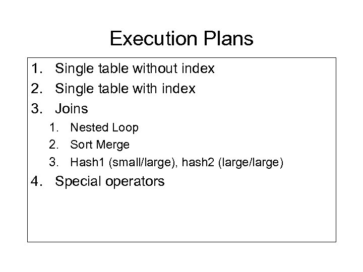 Execution Plans 1. Single table without index 2. Single table with index 3. Joins 1. Nested Loop 2. Sort Merge 3. Hash 1 (small/large), hash 2 (large/large) 4. Special operators
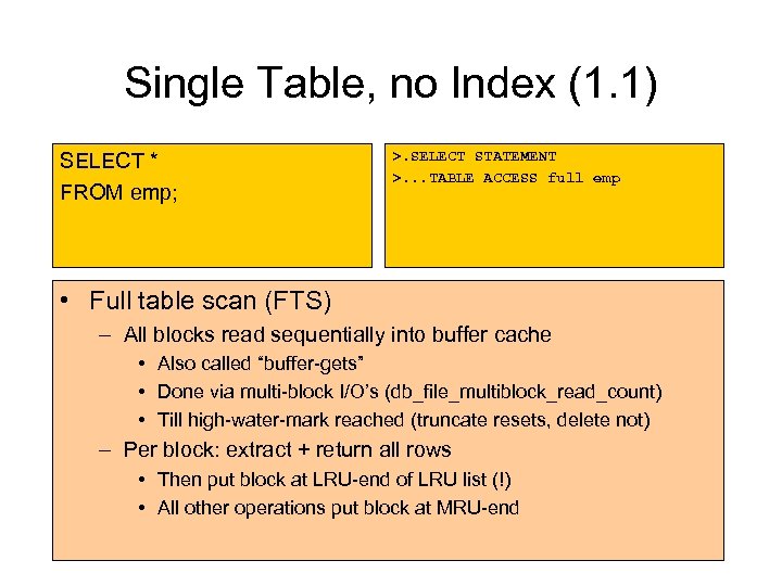 Single Table, no Index (1. 1) SELECT * FROM emp; >. SELECT STATEMENT >. . . TABLE ACCESS full emp • Full table scan (FTS) – All blocks read sequentially into buffer cache • Also called “buffer-gets” • Done via multi-block I/O’s (db_file_multiblock_read_count) • Till high-water-mark reached (truncate resets, delete not) – Per block: extract + return all rows • Then put block at LRU-end of LRU list (!) • All other operations put block at MRU-end
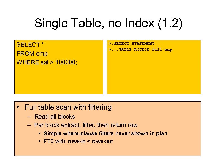 Single Table, no Index (1. 2) SELECT * FROM emp WHERE sal > 100000; >. SELECT STATEMENT >. . . TABLE ACCESS full emp • Full table scan with filtering – Read all blocks – Per block extract, filter, then return row • Simple where-clause filters never shown in plan • FTS with: rows-in < rows-out
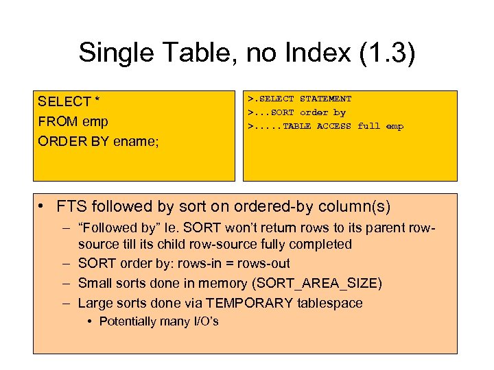 Single Table, no Index (1. 3) SELECT * FROM emp ORDER BY ename; >. SELECT STATEMENT >. . . SORT order by >. . . TABLE ACCESS full emp • FTS followed by sort on ordered-by column(s) – “Followed by” Ie. SORT won’t return rows to its parent rowsource till its child row-source fully completed – SORT order by: rows-in = rows-out – Small sorts done in memory (SORT_AREA_SIZE) – Large sorts done via TEMPORARY tablespace • Potentially many I/O’s
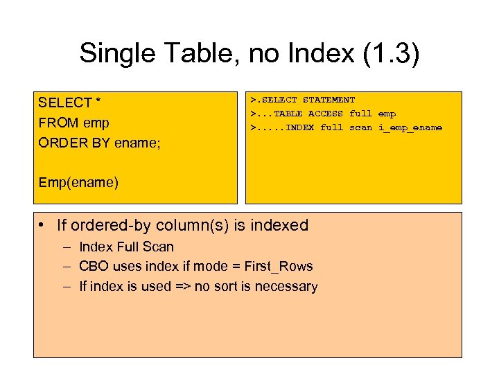 Single Table, no Index (1. 3) SELECT * FROM emp ORDER BY ename; >. SELECT STATEMENT >. . . TABLE ACCESS full emp >. . . INDEX full scan i_emp_ename Emp(ename) • If ordered-by column(s) is indexed – Index Full Scan – CBO uses index if mode = First_Rows – If index is used => no sort is necessary
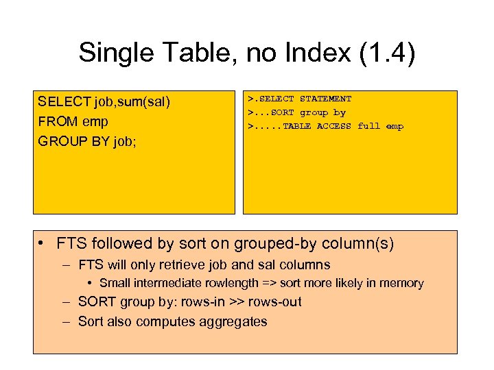 Single Table, no Index (1. 4) SELECT job, sum(sal) FROM emp GROUP BY job; >. SELECT STATEMENT >. . . SORT group by >. . . TABLE ACCESS full emp • FTS followed by sort on grouped-by column(s) – FTS will only retrieve job and sal columns • Small intermediate rowlength => sort more likely in memory – SORT group by: rows-in >> rows-out – Sort also computes aggregates
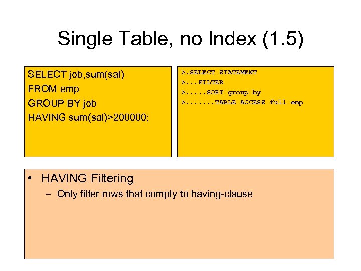 Single Table, no Index (1. 5) SELECT job, sum(sal) FROM emp GROUP BY job HAVING sum(sal)>200000; >. SELECT STATEMENT >. . . FILTER >. . . SORT group by >. . . . TABLE ACCESS full emp • HAVING Filtering – Only filter rows that comply to having-clause
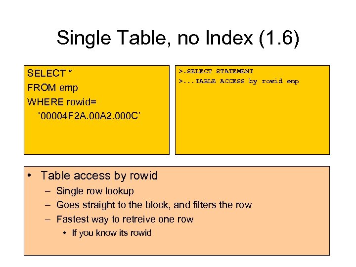 Single Table, no Index (1. 6) SELECT * FROM emp WHERE rowid= ‘ 00004 F 2 A. 00 A 2. 000 C’ >. SELECT STATEMENT >. . . TABLE ACCESS by rowid emp • Table access by rowid – Single row lookup – Goes straight to the block, and filters the row – Fastest way to retreive one row • If you know its rowid
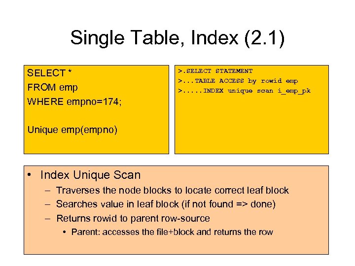 Single Table, Index (2. 1) SELECT * FROM emp WHERE empno=174; >. SELECT STATEMENT >. . . TABLE ACCESS by rowid emp >. . . INDEX unique scan i_emp_pk Unique emp(empno) • Index Unique Scan – Traverses the node blocks to locate correct leaf block – Searches value in leaf block (if not found => done) – Returns rowid to parent row-source • Parent: accesses the file+block and returns the row
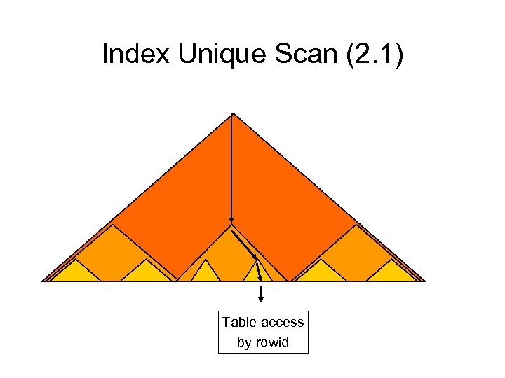 Index Unique Scan (2. 1) Table access by rowid
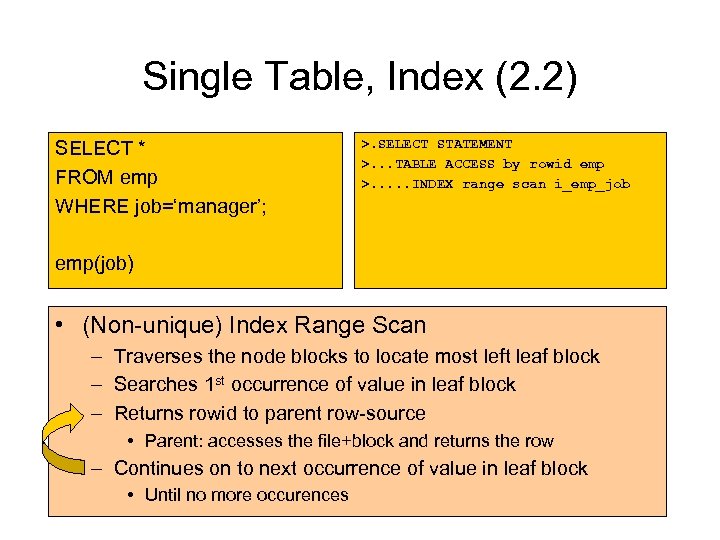 Single Table, Index (2. 2) SELECT * FROM emp WHERE job=‘manager’; >. SELECT STATEMENT >. . . TABLE ACCESS by rowid emp >. . . INDEX range scan i_emp_job emp(job) • (Non-unique) Index Range Scan – Traverses the node blocks to locate most left leaf block – Searches 1 st occurrence of value in leaf block – Returns rowid to parent row-source • Parent: accesses the file+block and returns the row – Continues on to next occurrence of value in leaf block • Until no more occurences
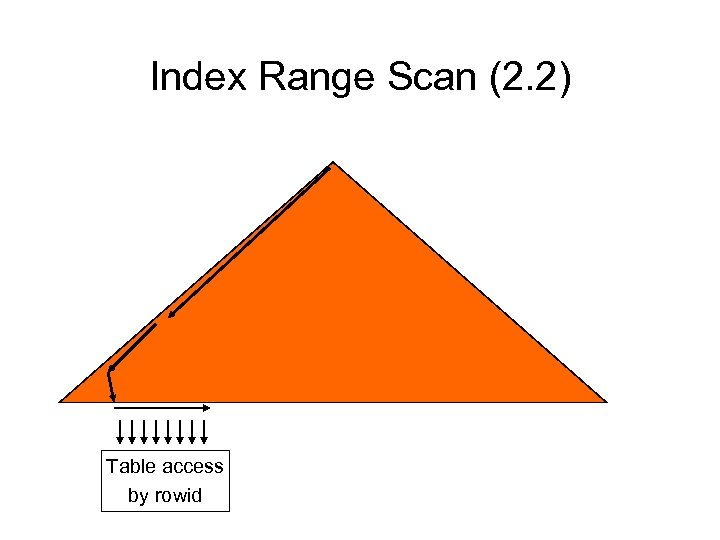 Index Range Scan (2. 2) Table access by rowid
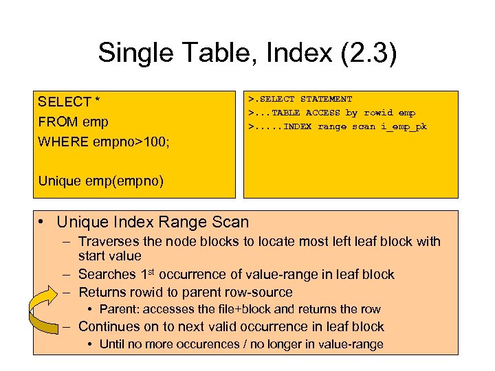 Single Table, Index (2. 3) SELECT * FROM emp WHERE empno>100; >. SELECT STATEMENT >. . . TABLE ACCESS by rowid emp >. . . INDEX range scan i_emp_pk Unique emp(empno) • Unique Index Range Scan – Traverses the node blocks to locate most left leaf block with start value – Searches 1 st occurrence of value-range in leaf block – Returns rowid to parent row-source • Parent: accesses the file+block and returns the row – Continues on to next valid occurrence in leaf block • Until no more occurences / no longer in value-range
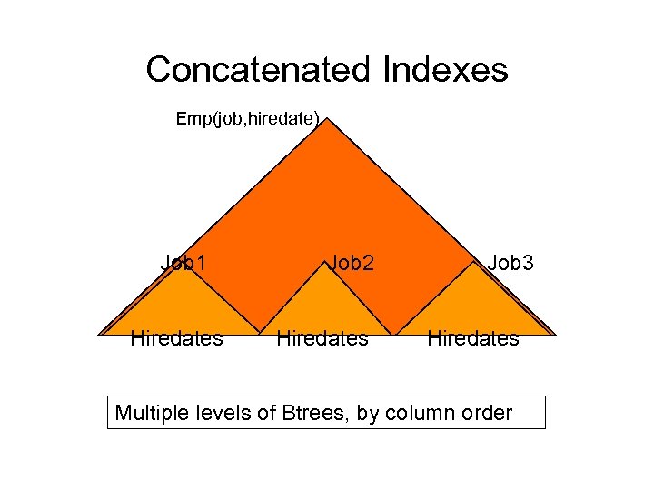 Concatenated Indexes Emp(job, hiredate) Job 1 Hiredates Job 2 Hiredates Job 3 Hiredates Multiple levels of Btrees, by column order
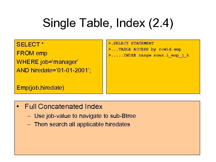 Single Table, Index (2. 4) SELECT * FROM emp WHERE job=‘manager’ AND hiredate=’ 01 -01 -2001’; >. SELECT STATEMENT >. . . TABLE ACCESS by rowid emp >. . . INDEX range scan i_emp_j_h Emp(job, hiredate) • Full Concatenated Index – Use job-value to navigate to sub-Btree – Then search all applicable hiredates
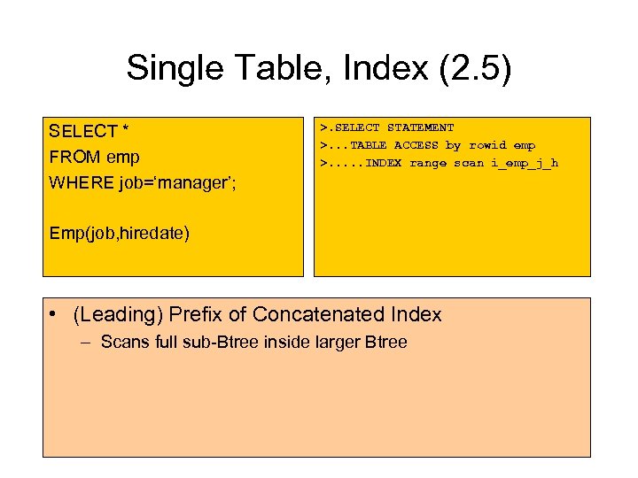 Single Table, Index (2. 5) SELECT * FROM emp WHERE job=‘manager’; >. SELECT STATEMENT >. . . TABLE ACCESS by rowid emp >. . . INDEX range scan i_emp_j_h Emp(job, hiredate) • (Leading) Prefix of Concatenated Index – Scans full sub-Btree inside larger Btree
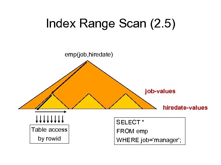 Index Range Scan (2. 5) emp(job, hiredate) job-values hiredate-values Table access by rowid SELECT * FROM emp WHERE job=‘manager’;
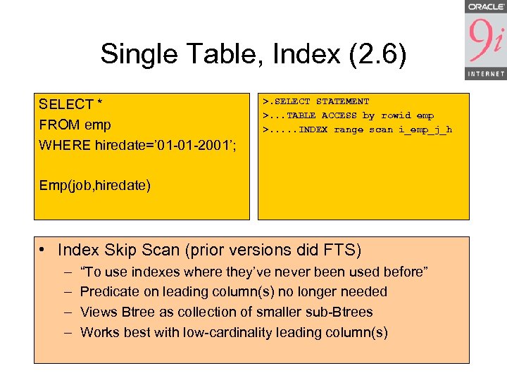 Single Table, Index (2. 6) SELECT * FROM emp WHERE hiredate=’ 01 -01 -2001’; >. SELECT STATEMENT >. . . TABLE ACCESS by rowid emp >. . . INDEX range scan i_emp_j_h Emp(job, hiredate) • Index Skip Scan (prior versions did FTS) – – “To use indexes where they’ve never been used before” Predicate on leading column(s) no longer needed Views Btree as collection of smaller sub-Btrees Works best with low-cardinality leading column(s)
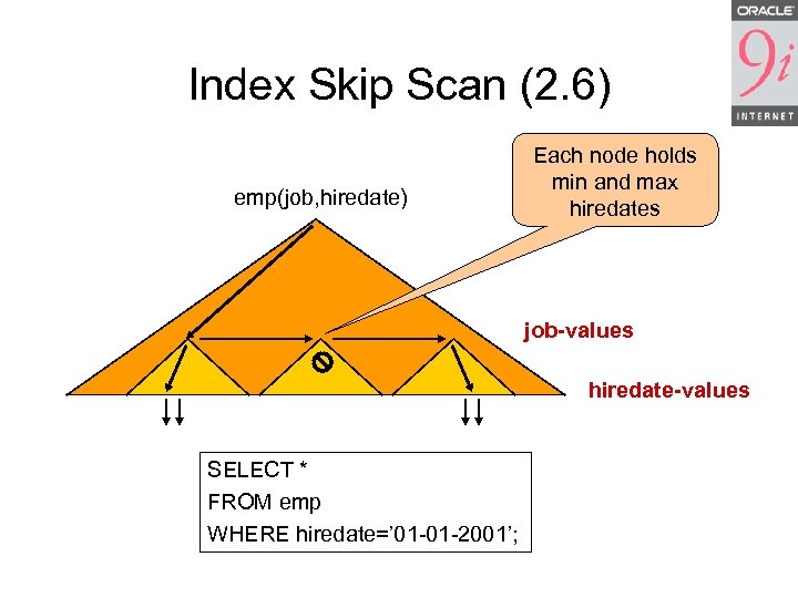 Index Skip Scan (2. 6) emp(job, hiredate) Each node holds min and max hiredates job-values hiredate-values SELECT * FROM emp WHERE hiredate=’ 01 -01 -2001’;
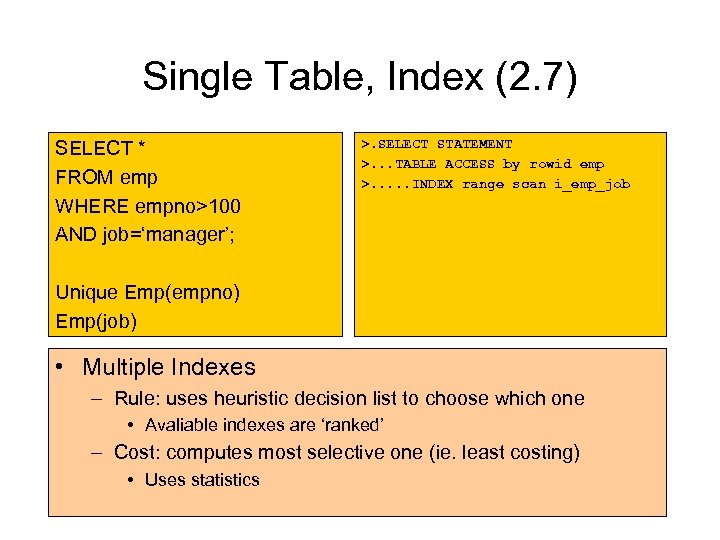 Single Table, Index (2. 7) SELECT * FROM emp WHERE empno>100 AND job=‘manager’; >. SELECT STATEMENT >. . . TABLE ACCESS by rowid emp >. . . INDEX range scan i_emp_job Unique Emp(empno) Emp(job) • Multiple Indexes – Rule: uses heuristic decision list to choose which one • Avaliable indexes are ‘ranked’ – Cost: computes most selective one (ie. least costing) • Uses statistics
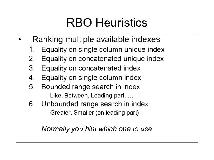 RBO Heuristics • Ranking multiple available indexes 1. 2. 3. 4. 5. Equality on single column unique index Equality on concatenated index Equality on single column index Bounded range search in index – Like, Between, Leading-part, … 6. Unbounded range search in index – Greater, Smaller (on leading part) Normally you hint which one to use
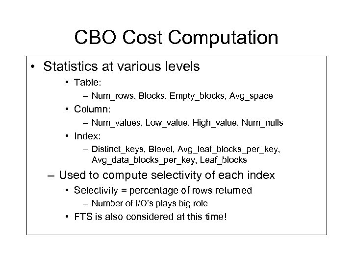 CBO Cost Computation • Statistics at various levels • Table: – Num_rows, Blocks, Empty_blocks, Avg_space • Column: – Num_values, Low_value, High_value, Num_nulls • Index: – Distinct_keys, Blevel, Avg_leaf_blocks_per_key, Avg_data_blocks_per_key, Leaf_blocks – Used to compute selectivity of each index • Selectivity = percentage of rows returned – Number of I/O’s plays big role • FTS is also considered at this time!
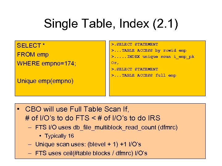 Single Table, Index (2. 1) SELECT * FROM emp WHERE empno=174; Unique emp(empno) >. SELECT STATEMENT >. . . TABLE ACCESS by rowid emp >. . . INDEX unique scan i_emp_pk Or, >. SELECT STATEMENT >. . . TABLE ACCESS full emp • CBO will use Full Table Scan If, # of I/O’s to do FTS < # of I/O’s to do IRS – FTS I/O uses db_file_multiblock_read_count (dfmrc) • Typically 16 – Unique scan uses: (blevel + 1) +1 I/O’s – FTS uses ceil(#table blocks / dfmrc) I/O’s
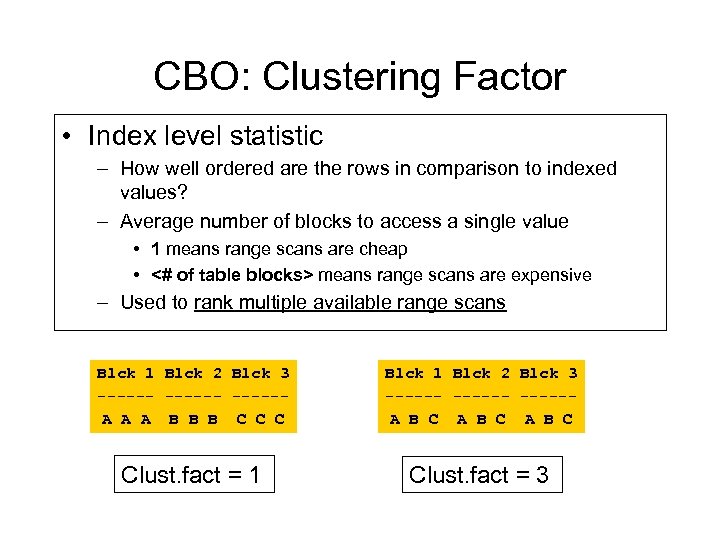 CBO: Clustering Factor • Index level statistic – How well ordered are the rows in comparison to indexed values? – Average number of blocks to access a single value • 1 means range scans are cheap • <# of table blocks> means range scans are expensive – Used to rank multiple available range scans Blck 1 Blck 2 Blck 3 ------A A A B B B C C C Blck 1 Blck 2 Blck 3 ------A B C Clust. fact = 1 Clust. fact = 3
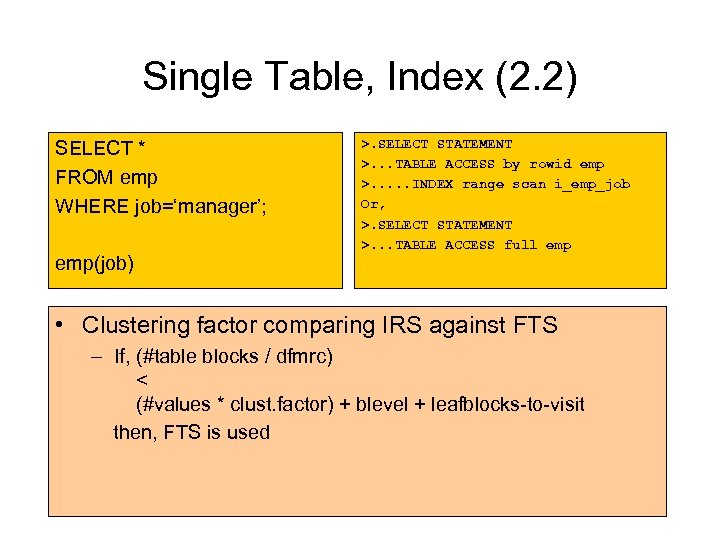 Single Table, Index (2. 2) SELECT * FROM emp WHERE job=‘manager’; emp(job) >. SELECT STATEMENT >. . . TABLE ACCESS by rowid emp >. . . INDEX range scan i_emp_job Or, >. SELECT STATEMENT >. . . TABLE ACCESS full emp • Clustering factor comparing IRS against FTS – If, (#table blocks / dfmrc) < (#values * clust. factor) + blevel + leafblocks-to-visit then, FTS is used
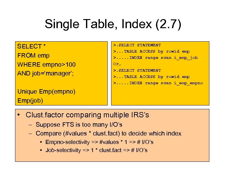 Single Table, Index (2. 7) SELECT * FROM emp WHERE empno>100 AND job=‘manager’; >. SELECT STATEMENT >. . . TABLE ACCESS by rowid emp >. . . INDEX range scan i_emp_job Or, >. SELECT STATEMENT >. . . TABLE ACCESS by rowid emp >. . . INDEX range scan i_empno Unique Emp(empno) Emp(job) • Clust. factor comparing multiple IRS’s – Suppose FTS is too many I/O’s – Compare (#values * clust. fact) to decide which index • Empno-selectivity => #values * 1 => # I/O’s • Job-selectivity => 1 * clust. fact => # I/O’s
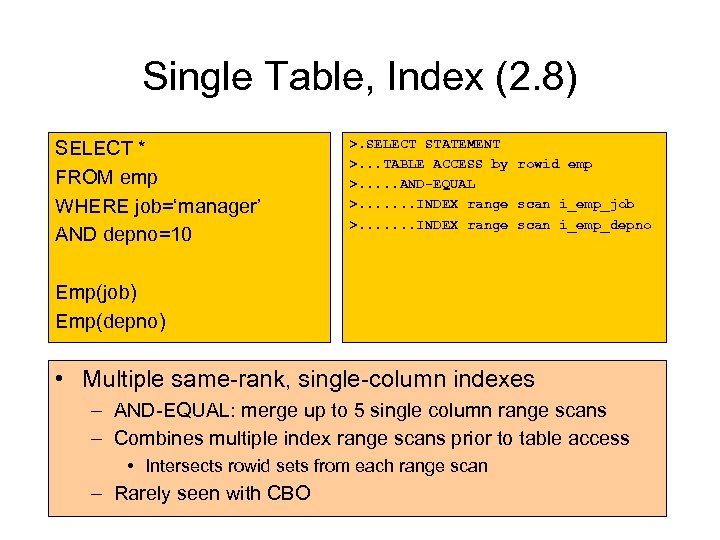 Single Table, Index (2. 8) SELECT * FROM emp WHERE job=‘manager’ AND depno=10 >. SELECT STATEMENT >. . . TABLE ACCESS by rowid emp >. . . AND-EQUAL >. . . . INDEX range scan i_emp_job >. . . . INDEX range scan i_emp_depno Emp(job) Emp(depno) • Multiple same-rank, single-column indexes – AND-EQUAL: merge up to 5 single column range scans – Combines multiple index range scans prior to table access • Intersects rowid sets from each range scan – Rarely seen with CBO
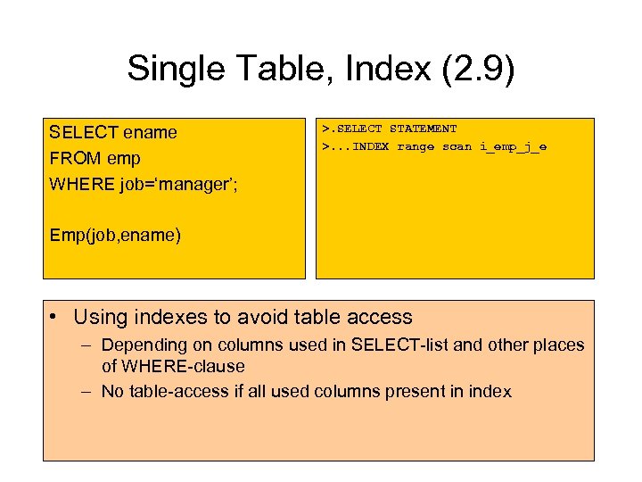 Single Table, Index (2. 9) SELECT ename FROM emp WHERE job=‘manager’; >. SELECT STATEMENT >. . . INDEX range scan i_emp_j_e Emp(job, ename) • Using indexes to avoid table access – Depending on columns used in SELECT-list and other places of WHERE-clause – No table-access if all used columns present in index
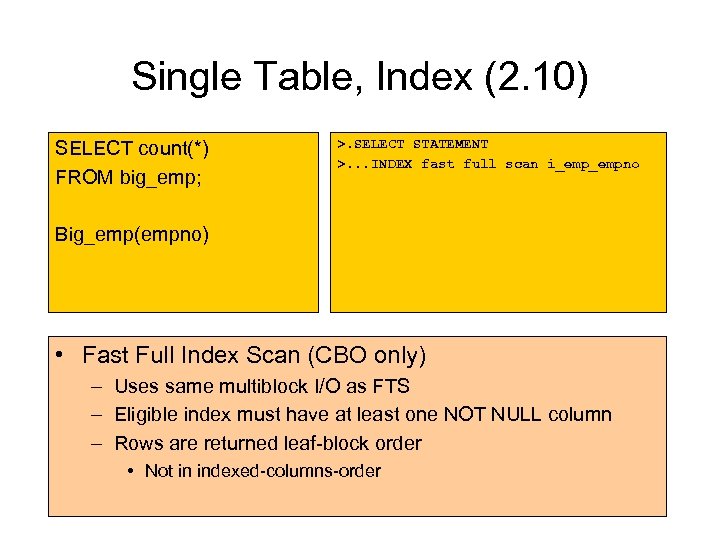 Single Table, Index (2. 10) SELECT count(*) FROM big_emp; >. SELECT STATEMENT >. . . INDEX fast full scan i_empno Big_emp(empno) • Fast Full Index Scan (CBO only) – Uses same multiblock I/O as FTS – Eligible index must have at least one NOT NULL column – Rows are returned leaf-block order • Not in indexed-columns-order
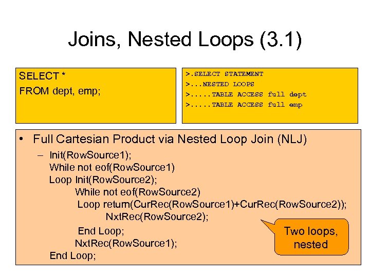 Joins, Nested Loops (3. 1) SELECT * FROM dept, emp; >. SELECT STATEMENT >. . . NESTED LOOPS >. . . TABLE ACCESS full dept >. . . TABLE ACCESS full emp • Full Cartesian Product via Nested Loop Join (NLJ) – Init(Row. Source 1); While not eof(Row. Source 1) Loop Init(Row. Source 2); While not eof(Row. Source 2) Loop return(Cur. Rec(Row. Source 1)+Cur. Rec(Row. Source 2)); Nxt. Rec(Row. Source 2); End Loop; Two loops, Nxt. Rec(Row. Source 1); nested End Loop;
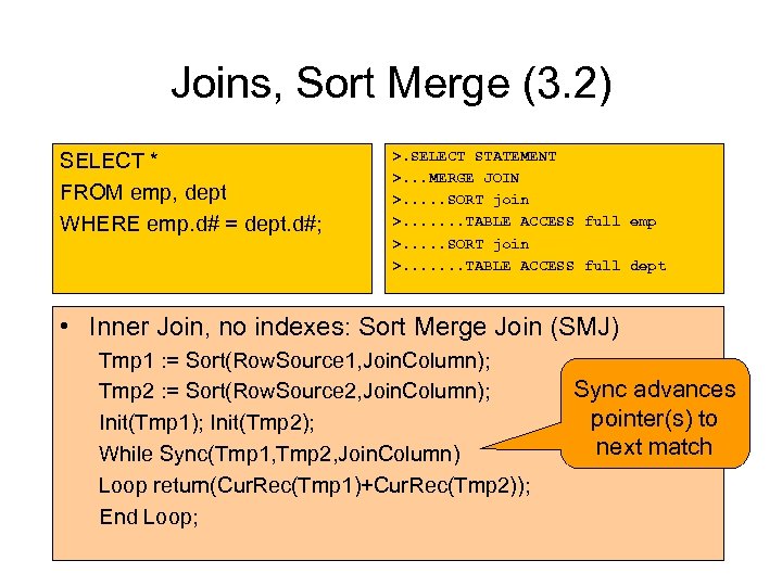 Joins, Sort Merge (3. 2) SELECT * FROM emp, dept WHERE emp. d# = dept. d#; >. SELECT STATEMENT >. . . MERGE JOIN >. . . SORT join >. . . . TABLE ACCESS full emp >. . . SORT join >. . . . TABLE ACCESS full dept • Inner Join, no indexes: Sort Merge Join (SMJ) Tmp 1 : = Sort(Row. Source 1, Join. Column); Tmp 2 : = Sort(Row. Source 2, Join. Column); Init(Tmp 1); Init(Tmp 2); While Sync(Tmp 1, Tmp 2, Join. Column) Loop return(Cur. Rec(Tmp 1)+Cur. Rec(Tmp 2)); End Loop; Sync advances pointer(s) to next match
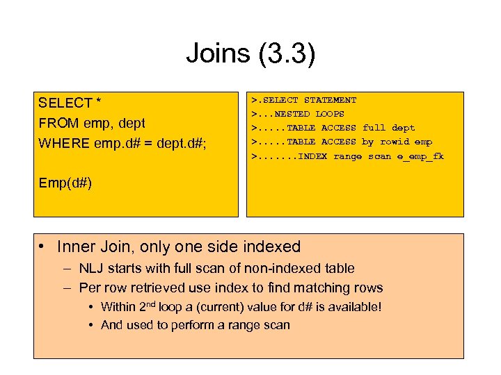 Joins (3. 3) SELECT * FROM emp, dept WHERE emp. d# = dept. d#; >. SELECT STATEMENT >. . . NESTED LOOPS >. . . TABLE ACCESS full dept >. . . TABLE ACCESS by rowid emp >. . . . INDEX range scan e_emp_fk Emp(d#) • Inner Join, only one side indexed – NLJ starts with full scan of non-indexed table – Per row retrieved use index to find matching rows • Within 2 nd loop a (current) value for d# is available! • And used to perform a range scan
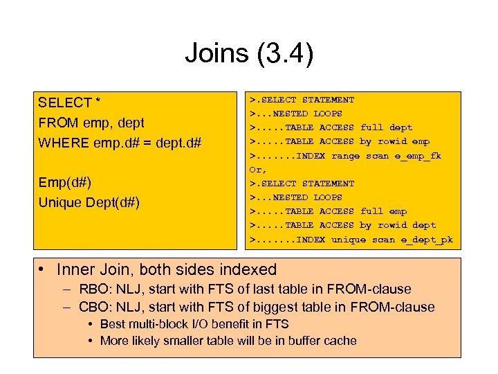 Joins (3. 4) SELECT * FROM emp, dept WHERE emp. d# = dept. d# Emp(d#) Unique Dept(d#) >. SELECT STATEMENT >. . . NESTED LOOPS >. . . TABLE ACCESS full dept >. . . TABLE ACCESS by rowid emp >. . . . INDEX range scan e_emp_fk Or, >. SELECT STATEMENT >. . . NESTED LOOPS >. . . TABLE ACCESS full emp >. . . TABLE ACCESS by rowid dept >. . . . INDEX unique scan e_dept_pk • Inner Join, both sides indexed – RBO: NLJ, start with FTS of last table in FROM-clause – CBO: NLJ, start with FTS of biggest table in FROM-clause • Best multi-block I/O benefit in FTS • More likely smaller table will be in buffer cache
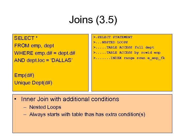 Joins (3. 5) SELECT * FROM emp, dept WHERE emp. d# = dept. d# AND dept. loc = ‘DALLAS’ >. SELECT STATEMENT >. . . NESTED LOOPS >. . . TABLE ACCESS full dept >. . . TABLE ACCESS by rowid emp >. . . . INDEX range scan e_emp_fk Emp(d#) Unique Dept(d#) • Inner Join with additional conditions – Nested Loops – Always starts with table thas extra condition(s)
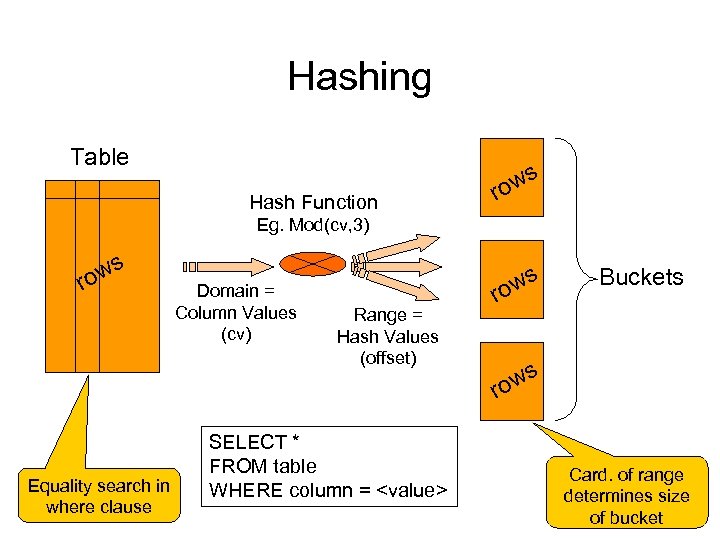 Hashing Table Hash Function ws ro Eg. Mod(cv, 3) ws ro Equality search in where clause Domain = Column Values (cv) Range = Hash Values (offset) SELECT * FROM table WHERE column =
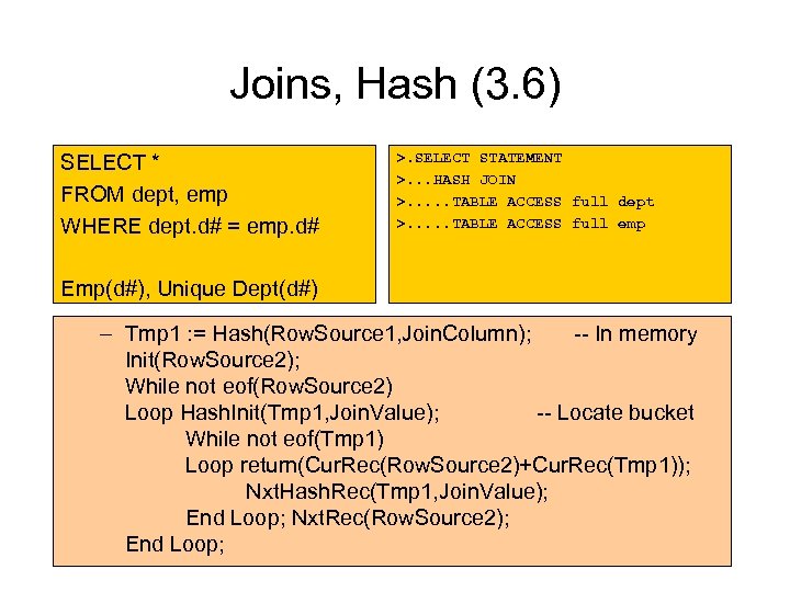 Joins, Hash (3. 6) SELECT * FROM dept, emp WHERE dept. d# = emp. d# >. SELECT STATEMENT >. . . HASH JOIN >. . . TABLE ACCESS full dept >. . . TABLE ACCESS full emp Emp(d#), Unique Dept(d#) – Tmp 1 : = Hash(Row. Source 1, Join. Column); -- In memory Init(Row. Source 2); While not eof(Row. Source 2) Loop Hash. Init(Tmp 1, Join. Value); -- Locate bucket While not eof(Tmp 1) Loop return(Cur. Rec(Row. Source 2)+Cur. Rec(Tmp 1)); Nxt. Hash. Rec(Tmp 1, Join. Value); End Loop; Nxt. Rec(Row. Source 2); End Loop;
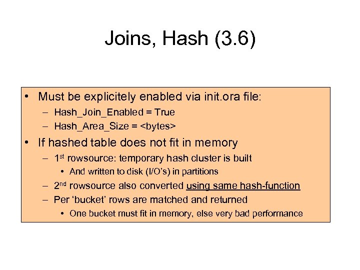 Joins, Hash (3. 6) • Must be explicitely enabled via init. ora file: – Hash_Join_Enabled = True – Hash_Area_Size =
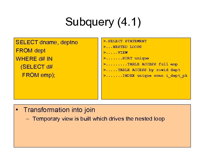 Subquery (4. 1) SELECT dname, deptno FROM dept WHERE d# IN (SELECT d# FROM emp); >. SELECT STATEMENT >. . . NESTED LOOPS >. . . VIEW >. . . . SORT unique >. . TABLE ACCESS full emp >. . . TABLE ACCESS by rowid dept >. . . . INDEX unique scan i_dept_pk • Transformation into join – Temporary view is built which drives the nested loop
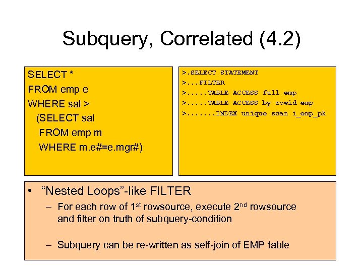 Subquery, Correlated (4. 2) SELECT * FROM emp e WHERE sal > (SELECT sal FROM emp m WHERE m. e#=e. mgr#) >. SELECT STATEMENT >. . . FILTER >. . . TABLE ACCESS full emp >. . . TABLE ACCESS by rowid emp >. . . . INDEX unique scan i_emp_pk • “Nested Loops”-like FILTER – For each row of 1 st rowsource, execute 2 nd rowsource and filter on truth of subquery-condition – Subquery can be re-written as self-join of EMP table
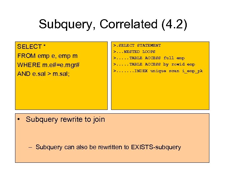 Subquery, Correlated (4. 2) SELECT * FROM emp e, emp m WHERE m. e#=e. mgr# AND e. sal > m. sal; >. SELECT STATEMENT >. . . NESTED LOOPS >. . . TABLE ACCESS full emp >. . . TABLE ACCESS by rowid emp >. . . . INDEX unique scan i_emp_pk • Subquery rewrite to join – Subquery can also be rewritten to EXISTS-subquery
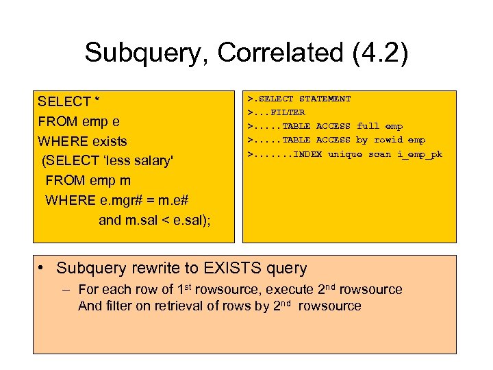 Subquery, Correlated (4. 2) SELECT * FROM emp e WHERE exists (SELECT ‘less salary' FROM emp m WHERE e. mgr# = m. e# and m. sal < e. sal); >. SELECT STATEMENT >. . . FILTER >. . . TABLE ACCESS full emp >. . . TABLE ACCESS by rowid emp >. . . . INDEX unique scan i_emp_pk • Subquery rewrite to EXISTS query – For each row of 1 st rowsource, execute 2 nd rowsource And filter on retrieval of rows by 2 nd rowsource
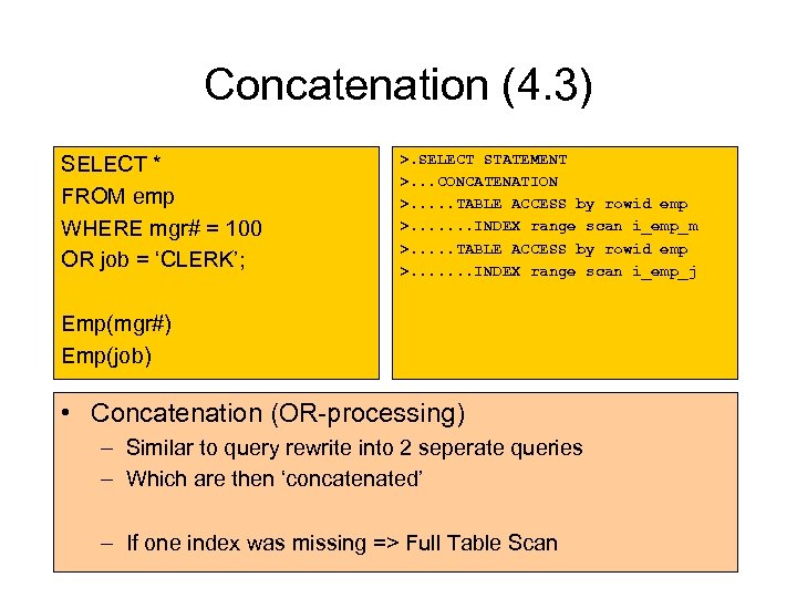 Concatenation (4. 3) SELECT * FROM emp WHERE mgr# = 100 OR job = ‘CLERK’; >. SELECT STATEMENT >. . . CONCATENATION >. . . TABLE ACCESS by rowid emp >. . . . INDEX range scan i_emp_m >. . . TABLE ACCESS by rowid emp >. . . . INDEX range scan i_emp_j Emp(mgr#) Emp(job) • Concatenation (OR-processing) – Similar to query rewrite into 2 seperate queries – Which are then ‘concatenated’ – If one index was missing => Full Table Scan
 Inlist Iterator (4. 4) SELECT * FROM dept WHERE d# in (10, 20, 30); >. SELECT STATEMENT >. . . INLIST ITERATOR >. . . TABLE ACCESS by rowid dept >. . . . INDEX unique scan i_dept_pk Unique Dept(d#) • Iteration over enumerated value-list – Every value executed seperately • Same as concatenation of 3 “OR-red” values
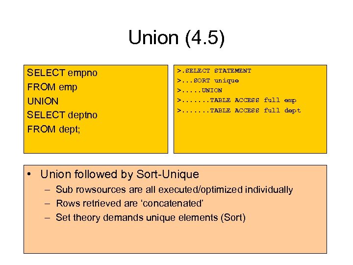 Union (4. 5) SELECT empno FROM emp UNION SELECT deptno FROM dept; >. SELECT STATEMENT >. . . SORT unique >. . . UNION >. . . . TABLE ACCESS full emp >. . . . TABLE ACCESS full dept • Union followed by Sort-Unique – Sub rowsources are all executed/optimized individually – Rows retrieved are ‘concatenated’ – Set theory demands unique elements (Sort)
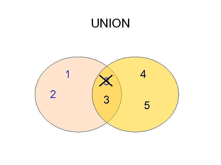 UNION 1 2 3 3 4 5
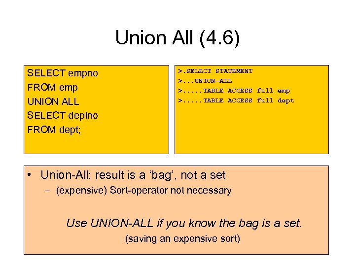 Union All (4. 6) SELECT empno FROM emp UNION ALL SELECT deptno FROM dept; >. SELECT STATEMENT >. . . UNION-ALL >. . . TABLE ACCESS full emp >. . . TABLE ACCESS full dept • Union-All: result is a ‘bag’, not a set – (expensive) Sort-operator not necessary Use UNION-ALL if you know the bag is a set. (saving an expensive sort)
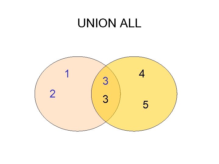 UNION ALL 1 2 3 3 4 5
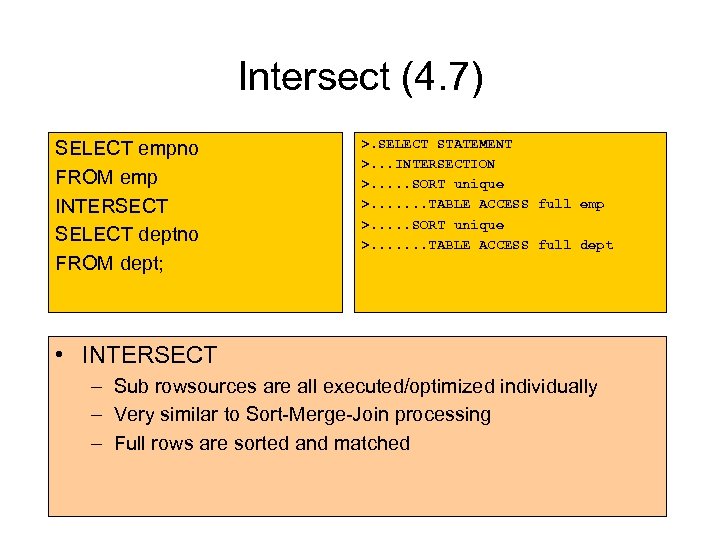 Intersect (4. 7) SELECT empno FROM emp INTERSECT SELECT deptno FROM dept; >. SELECT STATEMENT >. . . INTERSECTION >. . . SORT unique >. . . . TABLE ACCESS full emp >. . . SORT unique >. . . . TABLE ACCESS full dept • INTERSECT – Sub rowsources are all executed/optimized individually – Very similar to Sort-Merge-Join processing – Full rows are sorted and matched
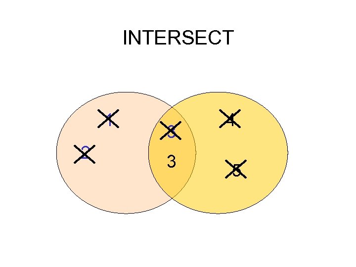 INTERSECT 1 2 3 3 4 5
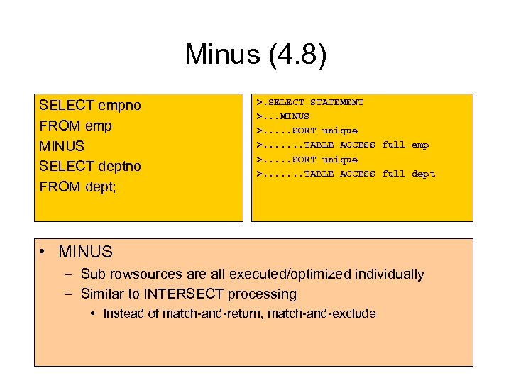 Minus (4. 8) SELECT empno FROM emp MINUS SELECT deptno FROM dept; >. SELECT STATEMENT >. . . MINUS >. . . SORT unique >. . . . TABLE ACCESS full emp >. . . SORT unique >. . . . TABLE ACCESS full dept • MINUS – Sub rowsources are all executed/optimized individually – Similar to INTERSECT processing • Instead of match-and-return, match-and-exclude
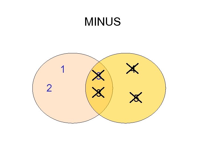 MINUS 1 2 3 3 4 5
 Break
Break
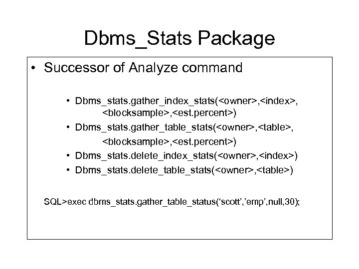
 Utilities • • Tracing SQL Hints Analyze command Dbms_Stats package
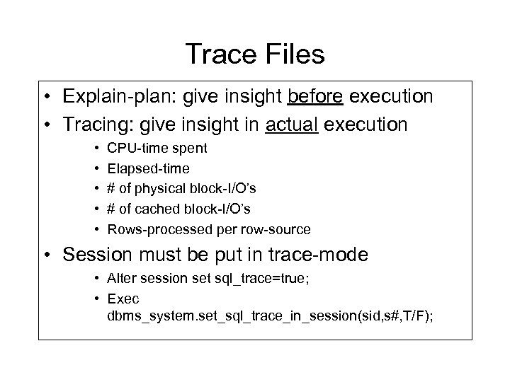 Trace Files • Explain-plan: give insight before execution • Tracing: give insight in actual execution • • • CPU-time spent Elapsed-time # of physical block-I/O’s # of cached block-I/O’s Rows-processed per row-source • Session must be put in trace-mode • Alter session set sql_trace=true; • Exec dbms_system. set_sql_trace_in_session(sid, s#, T/F);
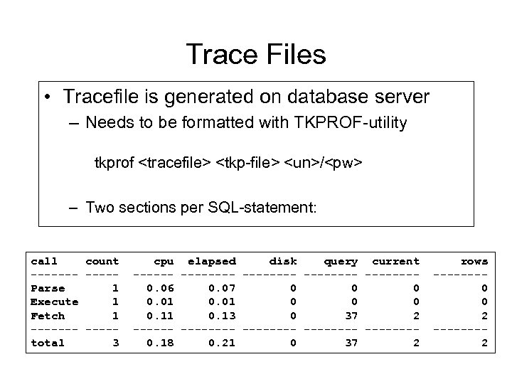 Trace Files • Tracefile is generated on database server – Needs to be formatted with TKPROF-utility tkprof
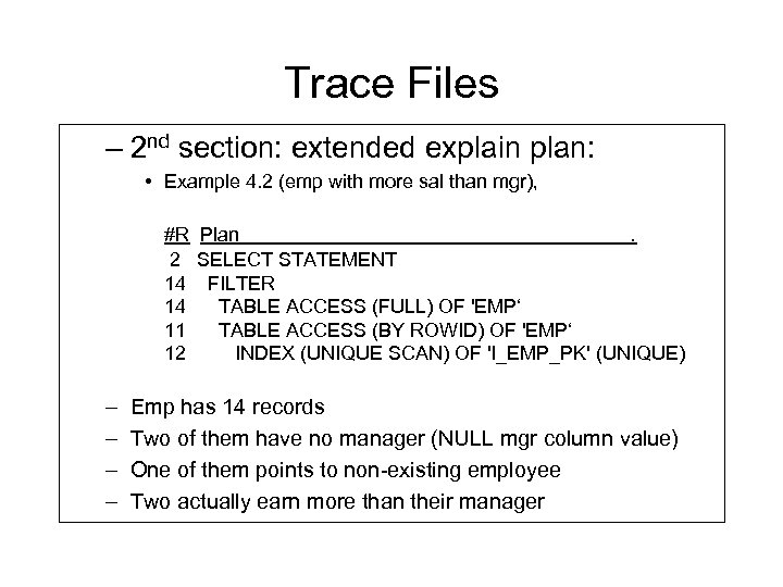 Trace Files – 2 nd section: extended explain plan: • Example 4. 2 (emp with more sal than mgr), #R Plan. 2 SELECT STATEMENT 14 FILTER 14 TABLE ACCESS (FULL) OF 'EMP‘ 11 TABLE ACCESS (BY ROWID) OF 'EMP‘ 12 INDEX (UNIQUE SCAN) OF 'I_EMP_PK' (UNIQUE) – – Emp has 14 records Two of them have no manager (NULL mgr column value) One of them points to non-existing employee Two actually earn more than their manager
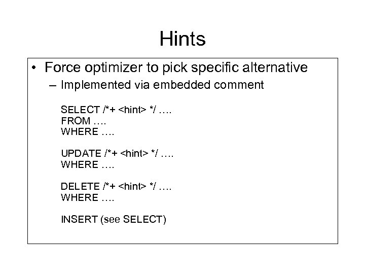 Hints • Force optimizer to pick specific alternative – Implemented via embedded comment SELECT /*+
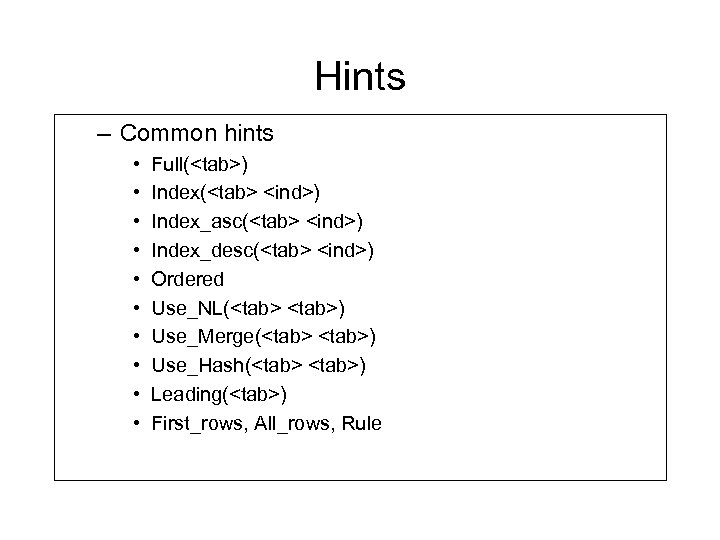 Hints – Common hints • • • Full(
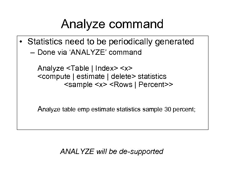 Analyze command • Statistics need to be periodically generated – Done via ‘ANALYZE’ command Analyze


