Example Rule 5 S 1 1

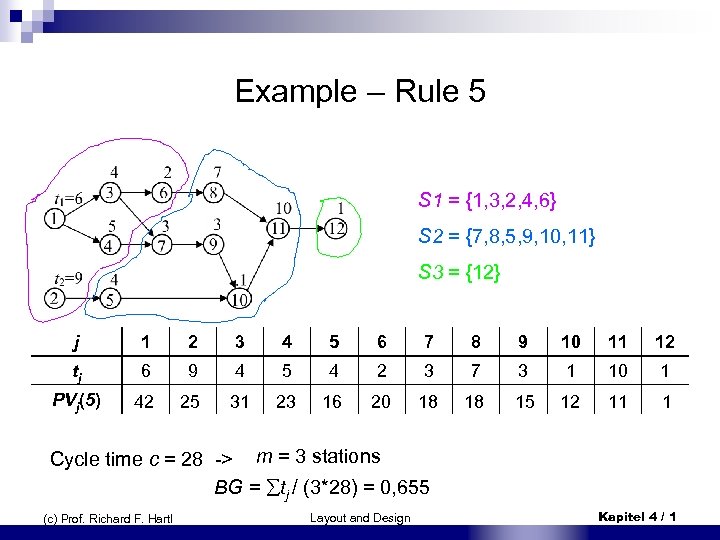Example – Rule 5 S 1 = {1, 3, 2, 4, 6} S 2 = {7, 8, 5, 9, 10, 11} S 3 = {12} j 1 2 3 4 5 6 7 8 9 10 11 12 tj 6 9 4 5 4 2 3 7 3 1 10 1 PVj(5) 42 25 31 23 16 20 18 18 15 12 11 1 Cycle time c = 28 -> m = 3 stations BG = tj / (3*28) = 0, 655 (c) Prof. Richard F. Hartl Layout and Design Kapitel 4 / 1

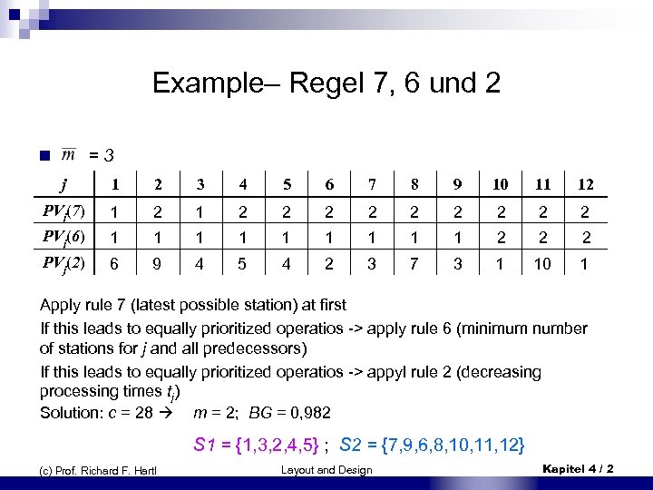Example– Regel 7, 6 und 2 n = 3 j 1 2 3 4 5 6 7 8 9 10 11 12 PVj(7) 1 2 2 2 2 2 PVj(6) 1 1 1 1 1 2 2 2 PVj(2) 6 9 4 5 4 2 3 7 3 1 10 1 Apply rule 7 (latest possible station) at first If this leads to equally prioritized operatios -> apply rule 6 (minimum number of stations for j and all predecessors) If this leads to equally prioritized operatios -> appyl rule 2 (decreasing processing times tj) Solution: c = 28 m = 2; BG = 0, 982 S 1 = {1, 3, 2, 4, 5} ; S 2 = {7, 9, 6, 8, 10, 11, 12} (c) Prof. Richard F. Hartl Layout and Design Kapitel 4 / 2

More heuristic methods n Stochastic elements for rules 2 to 7: Random selection of the next operation (out of the set of operations ready to be applied) ¨ Selection probabilities: proportional or reciprocally proportional to the priority value ¨ Randomly chosen priority rule ¨ n Enumerative heuristics: Determination of the set of all feasible assignments for the first station ¨ Choose the assignment leading to the minimum idle time ¨ Proceed the same way with the next station, and so on (greedy) ¨ (c) Prof. Richard F. Hartl Layout and Design Kapitel 4 / 3

Further heuristic methods n Heuristics for cutting&packing problems Precedence conditions have to be considered as well ¨ E. g. : generalization of first-fit-decreasing heuristic for the bin packing problem. ¨ n Shortest-path-problem with exponential number of nodes n Exchange methods: Exchange of operations between stations ¨ Objective: improvement in terms of the subordinate objective of equally utilized stations ¨ (c) Prof. Richard F. Hartl Layout and Design Kapitel 4 / 4

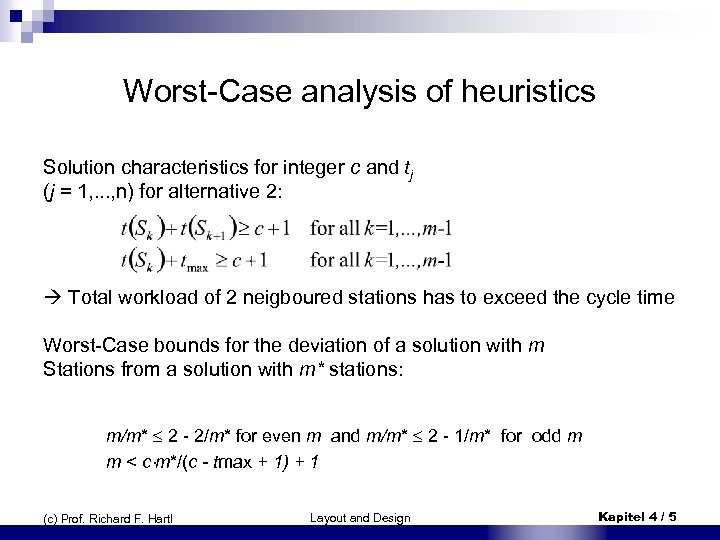Worst-Case analysis of heuristics Solution characteristics for integer c and tj (j = 1, . . . , n) for alternative 2: Total workload of 2 neigboured stations has to exceed the cycle time Worst-Case bounds for the deviation of a solution with m Stations from a solution with m* stations: m/m* 2 - 2/m* for even m and m/m* 2 - 1/m* for odd m m < c m*/(c - tmax + 1) + 1 (c) Prof. Richard F. Hartl Layout and Design Kapitel 4 / 5

Determination of cyle time c n Given number of stations n Cycle time unknown Minimize cycle time (alternative 1) or ¨ Optimize cycle time together with the number of stations trying to maximize the system´s efficiency (alternative 3). ¨ (c) Prof. Richard F. Hartl Layout and Design Kapitel 4 / 6

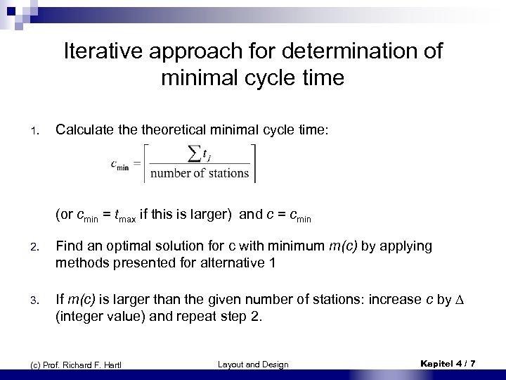Iterative approach for determination of minimal cycle time 1. Calculate theoretical minimal cycle time: (or cmin = tmax if this is larger) and c = cmin 2. Find an optimal solution for c with minimum m(c) by applying methods presented for alternative 1 3. If m(c) is larger than the given number of stations: increase c by (integer value) and repeat step 2. (c) Prof. Richard F. Hartl Layout and Design Kapitel 4 / 7

Iterative approach for determination of minimal cycle time n Repeat until feasible solution with cycle time c and number of stations m is found n If > 1, an interval reduction can be applied: if for c a solution with number of stations m has been found and for c- not, one can try to find a solution for c- /2 and so on… (c) Prof. Richard F. Hartl Layout and Design Kapitel 4 / 8

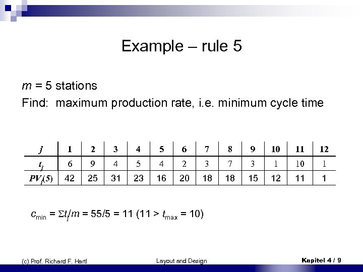Example – rule 5 m = 5 stations Find: maximum production rate, i. e. minimum cycle time j 1 2 3 4 5 6 7 8 9 10 11 12 tj 6 9 4 5 4 2 3 7 3 1 10 1 PVj(5) 42 25 31 23 16 20 18 18 15 12 11 1 cmin = tj/m = 55/5 = 11 (11 > tmax = 10) (c) Prof. Richard F. Hartl Layout and Design Kapitel 4 / 9

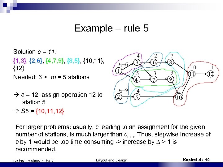Example – rule 5 Solution c = 11: {1, 3}, {2, 6}, {4, 7, 9}, {8, 5}, {10, 11}, {12} Needed: 6 > m = 5 stations c = 12, assign operation 12 to station 5 S 5 = {10, 11, 12} For larger problems: usually, c leading to an assignment for the given number of stations, is much larger than cmin. Thus, stepwise increase of c by 1 would be too time consuming -> increase by > 1 is recommended. (c) Prof. Richard F. Hartl Layout and Design Kapitel 4 / 10

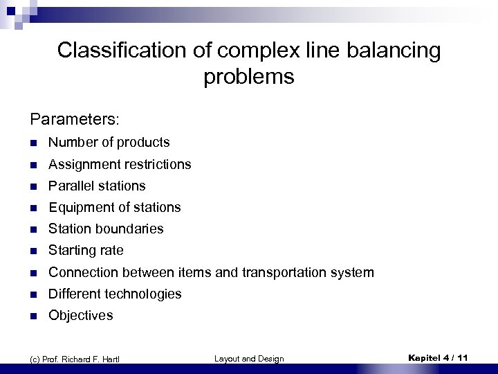Classification of complex line balancing problems Parameters: n Number of products n Assignment restrictions n Parallel stations n Equipment of stations n Station boundaries n Starting rate n Connection between items and transportation system n Different technologies n Objectives (c) Prof. Richard F. Hartl Layout and Design Kapitel 4 / 11

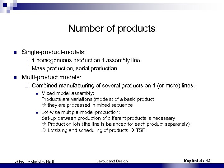Number of products n Single-product-models: 1 homogenuous product on 1 assembly line ¨ Mass production, serial production ¨ n Multi-product models: ¨ Combined manufacturing of several products on 1 (or more) lines. n n Mixed-model-assembly: Products are variations (models) of a basic product they are processed in mixed sequence Lot-wise multiple-model-production: Set-up between production of different products is necessary Production lots (the line is balanced for each product separately) Lotsizing and scheduling of products TSP (c) Prof. Richard F. Hartl Layout and Design Kapitel 4 / 12

Assignment restrictions n Restricted utilities: Stations have to be equipped with an adequate quantity of utilities ¨ Given environmental conditions ¨ n Positions: ¨ n Given positions of items within a station some operation may not be performed then (e. g. : underfloor operations) Operations: Minimum or maximum distances between 2 operations (concerning time or space) ¨ 2 operations may not be assigned to the same station ¨ n Qualifications: ¨ Combination of operations with similiar complexity (c) Prof. Richard F. Hartl Layout and Design Kapitel 4 / 13

Parallel stations n Models without parallel stations: ¨ n Heterogenuous stations with different operations serial line Models with parallel stations: At least 2 stations performing the same operation ¨ Alternating processing of 2 subsequent operations in parallel stations ¨ n Hybridization: Parallelization of operations: ¨ Assignment of an operation to 2 different stations of a serial line (c) Prof. Richard F. Hartl Layout and Design Kapitel 4 / 14

Equipment of stations n 1 -worker per station n Multiple workers per station: Different workloads between stations are possible ¨ Short-term capacity adaptions by using „jumpers“ ¨ n Fully automated stations: Workers are used for inspection of processes ¨ Workers are usually assigned to several stations ¨ (c) Prof. Richard F. Hartl Layout and Design Kapitel 4 / 15

Station boundaries n Closed stations: Expansion of station is limited ¨ Workers are not allowed to leave the station during processing ¨ n Open stations: Workers my leave their station in („rechtsoffen“) or in reversed („linksoffen“) flow direction of the line ¨ Short-term capacity adaption by under- and over-usage of cycle time. ¨ E. g. : Manufacturing of variations of products ¨ (c) Prof. Richard F. Hartl Layout and Design Kapitel 4 / 16

Starting rate n Models with fixed statrting rate: ¨ n Subsequent items enter the line after a fixed time span. Models with variable starting rate: An item enters the line once the first station of the line is idle ¨ Distances between items on the line may vary (in case of multipleproduct-production) ¨ (c) Prof. Richard F. Hartl Layout and Design Kapitel 4 / 17

Connection between items and transportation systems n Unmoveable items: Items are attached to the transportation system and may not be removed ¨ Maybe turning moves are possible ¨ n Moveable items: ¨ Removing items from the transportation system during processing is n n ¨ Post-production Intermediate inventories Flow shop production without fixed time constraints for each station (c) Prof. Richard F. Hartl Layout and Design Kapitel 4 / 18

Different technologies n Given production technologies ¨ n Schedules are given Different technologies Production technology is to be chosen ¨ Different alternative schedules are given (precedence graph) and/or ¨ ¨ different processing times for 1 operation (c) Prof. Richard F. Hartl Layout and Design Kapitel 4 / 19

Objectives n Time-oriented objectives Minimization of total cycle time, total idle time, ratio of idle time, total waiting time ¨ Maximization of capacity utilization (system`s efficieny) – most relevant for (single-product) problems ¨ Equally utilized stations ¨ n Further objectives Minimization of number of stations in case of given cycle time ¨ Minimization of cycle time in case of given number of stations ¨ Minimization of sum of weighted cycle time and weighted number of stations ¨ (c) Prof. Richard F. Hartl Layout and Design Kapitel 4 / 20

Objectives n Profit-oriented approaches: Maximization of total marginal return ¨ Minimization of total costs ¨ n n Machines- and utility costs (hourly wage rate of machines depends on the number of stations) Labour costs: often identical rates of labour costs for all workers in all stations) Material costs: defined by output quantity and cycle time Idle time costs: Opportunity costs – depend on cycle time and number of stations (c) Prof. Richard F. Hartl Layout and Design Kapitel 4 / 21

Multiple-product-problems Mixed model assembly: Several variants of a basic product are processed in mixed sequence on a production line. n Processing times of operations may vary between the models n Some operations may not be necessary for all of the variants Determination of an optimal line balancing and of an optimal sequence of models. n (c) Prof. Richard F. Hartl Layout and Design Kapitel 4 / 22

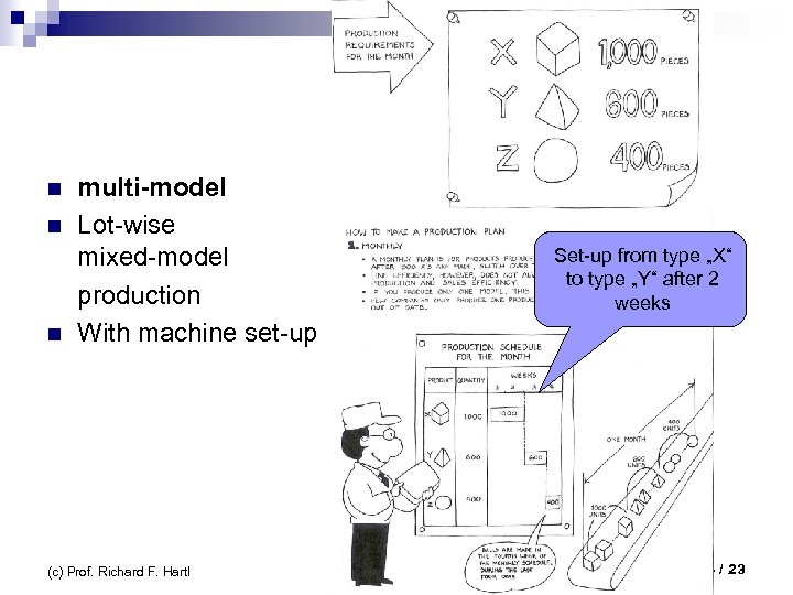n n n multi-model Lot-wise mixed-model production With machine set-up (c) Prof. Richard F. Hartl Set-up from type „X“ to type „Y“ after 2 weeks Layout and Design Kapitel 4 / 23

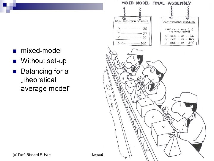n n n mixed-model Without set-up Balancing for a „theoretical average model“ (c) Prof. Richard F. Hartl Layout and Design Kapitel 4 / 24

Balancing mixed-model assembly lines n Similiar models: Avoid set-ups and lot sizing ¨ Consider all models simultaneously ¨ n Generalization of the basic model ¨ ¨ ¨ Production of p models of 1 basic model with up to n operations; production method is given Given precedence conditions for operations in each model j = 1, . . . , n aggregated precendence graph for all models Each operation is assigned to exactly 1 station Given processing times tjv for each operation j in each model v Given demand bv for each model v Given total time T of the working shifts in the planning horizon (c) Prof. Richard F. Hartl Layout and Design Kapitel 4 / 25

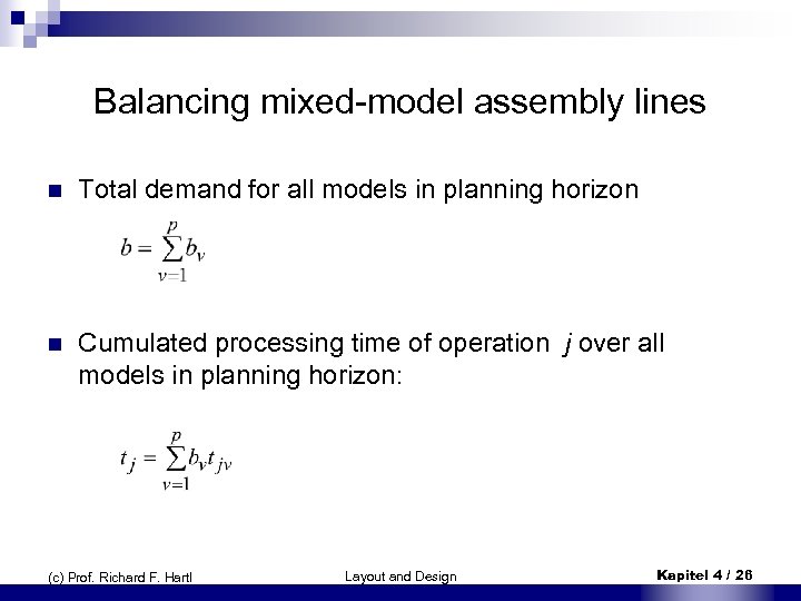Balancing mixed-model assembly lines n Total demand for all models in planning horizon n Cumulated processing time of operation j over all models in planning horizon: (c) Prof. Richard F. Hartl Layout and Design Kapitel 4 / 26

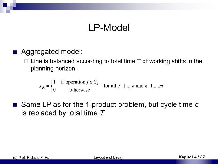LP-Model n Aggregated model: ¨ n Line is balanced according to total time T of working shifts in the planning horizon. Same LP as for the 1 -product problem, but cycle time c is replaced by total time T (c) Prof. Richard F. Hartl Layout and Design Kapitel 4 / 27

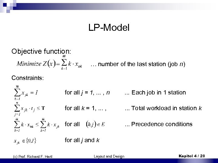LP-Model Objective function: … number of the last station (job n) Constraints: for all j = 1, . . . , n (c) Prof. Richard F. Hartl for all k = 1, . . . , . . . Total workload in station k for all . . . Each job in 1 station . . . Precedence conditions for all j and k Layout and Design Kapitel 4 / 28

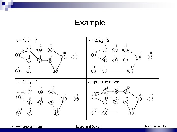Example v = 1, b 1 = 4 v = 2, b 2 = 2 v = 3, b 3 = 1 aggregated model (c) Prof. Richard F. Hartl Layout and Design Kapitel 4 / 29

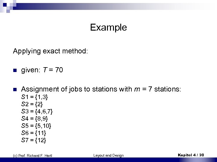Example Applying exact method: n given: T = 70 n Assignment of jobs to stations with m = 7 stations: S 1 = {1, 3} S 2 = {2} S 3 = {4, 6, 7} S 4 = {8, 9} S 5 = {5, 10} S 6 = {11} S 7 = {12} (c) Prof. Richard F. Hartl Layout and Design Kapitel 4 / 30

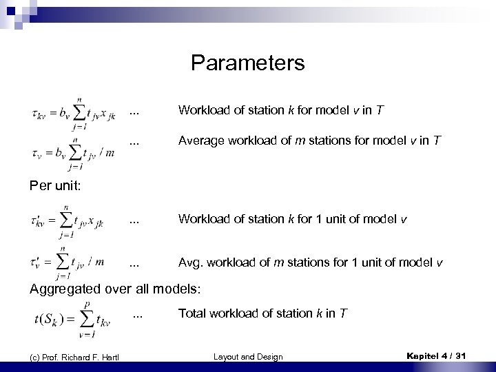Parameters. . . Workload of station k for model v in T . . . Average workload of m stations for model v in T . . . Workload of station k for 1 unit of model v . . . Avg. workload of m stations for 1 unit of model v Per unit: Aggregated over all models: . . . (c) Prof. Richard F. Hartl Total workload of station k in T Layout and Design Kapitel 4 / 31

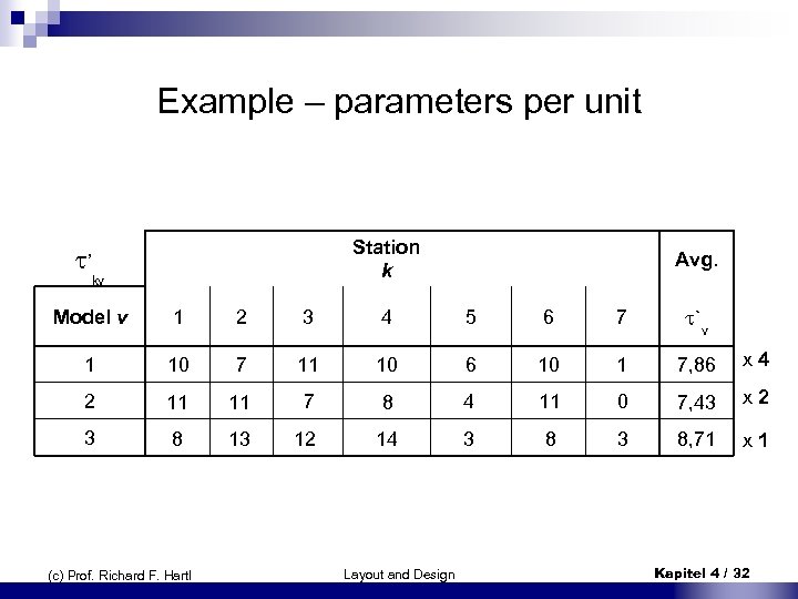Example – parameters per unit Station k Avg. Model v 1 2 3 4 5 6 7 `v 1 10 7 11 10 6 10 1 7, 86 x 4 2 11 11 7 8 4 11 0 7, 43 x 2 3 8 13 12 14 3 8, 71 x 1 ’ kv (c) Prof. Richard F. Hartl Layout and Design Kapitel 4 / 32

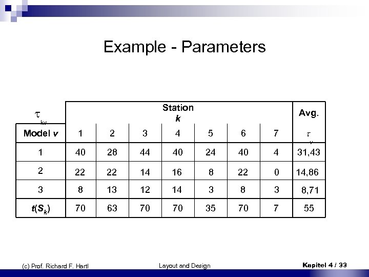Example - Parameters Station k Avg. 1 2 3 4 5 6 7 kv Model v v 1 40 28 44 40 24 40 4 31, 43 2 22 22 14 16 8 22 0 14, 86 3 8 13 12 14 3 8, 71 t(Sk) 70 63 70 70 35 70 7 55 (c) Prof. Richard F. Hartl Layout and Design Kapitel 4 / 33

Conclusion n Station 5 and 7 are not efficiently utilized n Variation of workload kv of stations k is higher for the models v as for the aggregated model t(Sk) n Parameters per unit show a high degree of variation for the models. Model 3, for example, leads to an high utilization of stations 2, 3, and 4. ¨ If we want to produce several units of model 3 subsequently, the average cycle time will be exceeded -> the line has to be stopped (c) Prof. Richard F. Hartl Layout and Design Kapitel 4 / 34

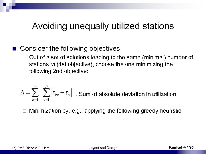Avoiding unequally utilized stations n Consider the following objectives ¨ Out of a set of solutions leading to the same (minimal) number of stations m (1 st objective), choose the one minimizing the following 2 nd objective: . . . Sum of absolute deviation in utilization ¨ Minimization by, e. g. , applying the following greedy heuristic (c) Prof. Richard F. Hartl Layout and Design Kapitel 4 / 35

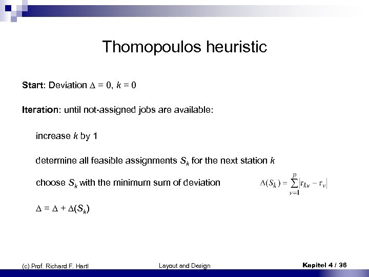Thomopoulos heuristic Start: Deviation = 0, k = 0 Iteration: until not-assigned jobs are available: increase k by 1 determine all feasible assignments Sk for the next station k choose Sk with the minimum sum of deviation = + (Sk) (c) Prof. Richard F. Hartl Layout and Design Kapitel 4 / 36

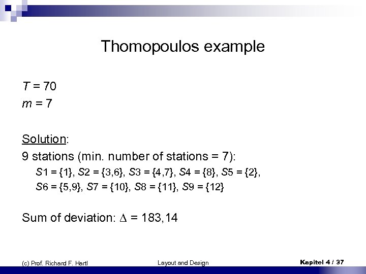Thomopoulos example T = 70 m = 7 Solution: 9 stations (min. number of stations = 7): S 1 = {1}, S 2 = {3, 6}, S 3 = {4, 7}, S 4 = {8}, S 5 = {2}, S 6 = {5, 9}, S 7 = {10}, S 8 = {11}, S 9 = {12} Sum of deviation: = 183, 14 (c) Prof. Richard F. Hartl Layout and Design Kapitel 4 / 37

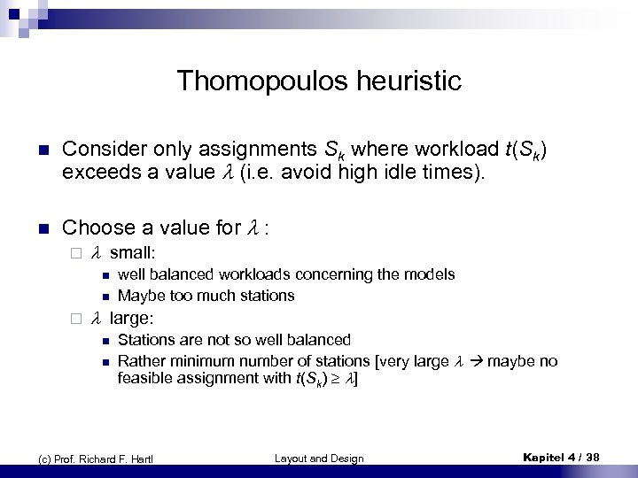Thomopoulos heuristic n Consider only assignments Sk where workload t(Sk) exceeds a value (i. e. avoid high idle times). n Choose a value for : ¨ small: n n ¨ well balanced workloads concerning the models Maybe too much stations large: n n Stations are not so well balanced Rather minimum number of stations [very large maybe no feasible assignment with t(Sk) ] (c) Prof. Richard F. Hartl Layout and Design Kapitel 4 / 38

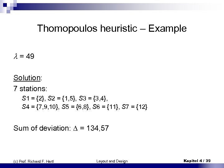Thomopoulos heuristic – Example = 49 Solution: 7 stations: S 1 = {2}, S 2 = {1, 5}, S 3 = {3, 4}, S 4 = {7, 9, 10}, S 5 = {6, 8}, S 6 = {11}, S 7 = {12} Sum of deviation: = 134, 57 (c) Prof. Richard F. Hartl Layout and Design Kapitel 4 / 39

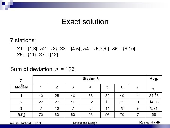Exact solution 7 stations: S 1 = {1, 3}, S 2 = {2}, S 3 = {4, 5}, S 4 = {6, 7, 9 }, S 5 = {8, 10}, S 6 = {11}, S 7 = {12} Sum of deviation: = 126 Station k Avg. Modelv 1 2 3 4 5 6 7 1 40 28 40 36 32 40 4 31, 43 2 22 22 16 12 10 22 0 14, 86 3 8 13 7 8 14 8 3 8, 71 t(Sk) 70 63 63 56 56 70 7 55 kv (c) Prof. Richard F. Hartl Layout and Design v Kapitel 4 / 40

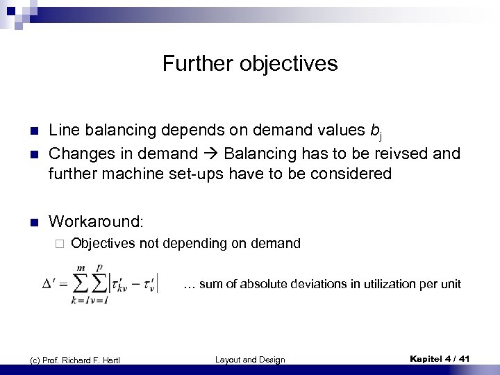Further objectives n Line balancing depends on demand values bj Changes in demand Balancing has to be reivsed and further machine set-ups have to be considered n Workaround: n ¨ Objectives not depending on demand … sum of absolute deviations in utilization per unit (c) Prof. Richard F. Hartl Layout and Design Kapitel 4 / 41

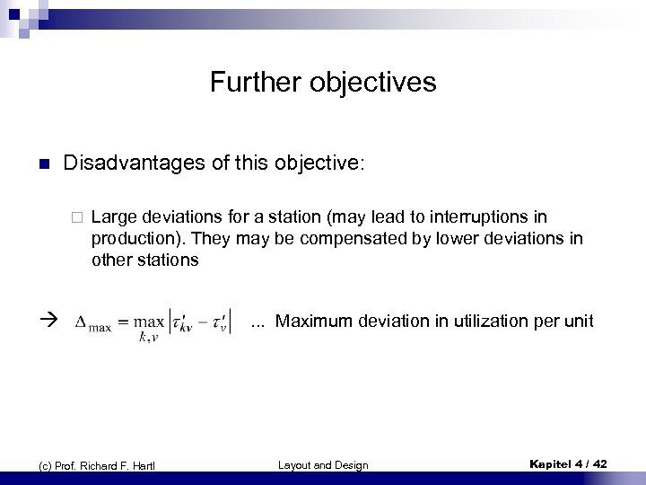Further objectives n Disadvantages of this objective: ¨ Large deviations for a station (may lead to interruptions in production). They may be compensated by lower deviations in other stations (c) Prof. Richard F. Hartl . . . Maximum deviation in utilization per unit Layout and Design Kapitel 4 / 42