Example — HW Let us design a

Example - HW • Let us design a database for a Student Record System, including information about these Entities Students, Fees, Course, Textbooks and Department. • Conceptual Design: – Draw the E/R diagram for this database. – Work out the type of relationships among the entities • Logical Design – Work out what the attributes of each entity • See if you can convert this Database into Access.

E-R Model of a student database Students pay Fees Courses Enrol in has Textbooks offer Department

Types of relationships • • • Student and Course – many to many Students and Fees – one to one Textbooks and Fees – one to one Department and Courses – one to many Course and Textbooks – one to many – One to One (1 ------m) – One to Many – Many to Many

Relationships • One – one relationship, an entity of either set can be associated with at most one entity of the other set; • Many – one relationship, each entity of the many side is associated with at most one entity of the other side; • Many – many relationships; place no restriction on the multiplicity.

Logical Design - Attributes • Students (Idnumber, surname, fname, gender, contact, sponsor • Department. Courses (Course. Number, Department. Id, Course Title, Coordinator) • Textbook. Fees(Fee. Code, ISBN, Fee) • Departments(Depatment. Id, Department name) • Course. Textbooks(ISBN, Course number, Title, Author, Edition) • Student. Courses(Idnumber, Course. Number, Fees. Id)

Record Types • Now that we have the attributes of our entities, we will refer to them as record types. The record types are linked together by key fields which are highlighted in bold.

Physical Design • Once we have identified our record types and the relationship between the record type and the fields, the next step is to create tables. • To create tables we need a DBMS. • The DDL part of the DBMS enables us to create tables, alter, or delete a no longer needed table.

Table Student Data Definition Language (DDL) : Idnumber Surname Fname Gener Sponsor Char (10) NOT NULL Char (30) Char (1) Char (30)

Instances of an E/R Diagram • E/R diagrams are a document for describing the schema of database, that is their structure; • A database described by an E/R diagram will contain particular data, which we call the database instance. • Specifically, for each entity set, the database instance will have a particular finite set of entities. Each of these entities has particular values for each attribute.

Multiplicity of Binary E/R Diagram • In general, a binary relationship can connect any member of one of its entity sets to any number of members of the other entity set. • Suppose R is a relationship connecting entity sets E and F, Then: • If each member of E can be connected by R to at most one member of F then we say that R is Many – One from E to F. • Note that in a many to one relationship from E to F, each entity in f can be connected to many members of E

Multiway Relationships • A multiway relationship in an E/R diagram that is represented by lines from the relationship diamond to each of the involved entity sets. • A studio has contracted with a particular star to act in a particular movie. Stars Contracts Studios Movies

Roles in Relationships • One role is original and the other is Sequel indicating the original movie and its sequel respectively. • We assume that a movie may have many sequels, but for each sequel that is only one original movie. • Thus the relationship is many to one from Sequel movies to Original movies. original Movies Sequel-of sequel

Attributes on Relationships • Sometime it is convenient, or even essential, to associate attributes with a relationship, rather than with any one of the entity sets that relationship connects. Salary Movies Contracts Studios Stars

Summary • • Data Modeling SDLC What is Data Modeling Application Audience and Services Entities Attributes Relationships Entity Relationship Diagrams

Data Modeling 2

Database Modeling & Implementation Process Ideas E/R Design Relational Schema Relational Database

Elements of E/R Model • Entity sets • Attributes • Relationships

Data Modeling To draw a data model we follow the following informal Rules - Identify all the candidate entity types Identify for each entity type the attributes involved Identify for each relationship type the attributes involved Put constraints on each relationship type (i. e (a) cardinality, (b) participation

Data Modeling - Entity • Two rules of “thumb” to help in identifying Entity and Relationship type are: - An Entity type corresponds to NOUN - A Relationship type corresponds to VERB

Data Modeling - Entity • Entity Sets - An entity is an abstract object of some sort and a collection of similar entities forms an Entity Set • E. g. * Employee entity set consists of the set of all employees » Department entity set consists of the set of all departments

Data Modeling - Attributes • Entity Sets have associated attributes, which are properties of the entity in that set E. g. Entity Set Movies might be given attributes such as title ( the name of the movie) or length (duration of the movie)

Data Modeling - Attributes • Most attributes are single – valued i. e. they have a single value for a given entity eg Age • However some attributes are multi-valued e. g. Tihe Certificate attribute for an employee can be multi-valued

Data Modeling - Attributes • Attributes which composed of several basic attributes are composite. Address Street Address Number Street Name City District

Data Modeling - Attributes • Attributes can also be null-valued e. g. tihe certificate attribute for a non graduate student take a null value • Null values can arise in two different contexts - when the attribute is not applicable - when the attribute is applicable, but the value is unknown • All entities that have the same attributes are classified as entity types

Data Modeling - Relationships Link or association between two or more entities - i. e. connections among two or more entity sets E. g. the fact that Ana works for the Accounting department represent a relationship work for between Ana and Accounting Department A relationship type is the set of all relationships between one or more entity types

Data Modeling - Relationships • Employee E 1 E 2 E 3 E 4 E 5 E 6 E 7 Works For R 1 R 2 R 3 R 4 R 5 R 6 R 7 Dept D 1 D 2 D 3 D 4

Data Modeling - Relationships • The Degree of a relationship type is the number of participating entity types • The set of all occurrences of WORK-FOR relationship make up the WORK-FOR relationship type

Recursive Relationship • These are relationship types of degree 1 • E. g. an employee has a supervisor who is in turn is an employee SUPERVISOR EMPLOYEE

Cardinality • Constraints on Relationship Types Cardinality - specifies the number of relationships that an entity can participate in

Cardinality • Employee Manages E 1 E 2 E 3 E 4 E 5 E 6 E 7 • R 1 R 2 R 3 R 4 Dept D 1 D 2 D 3 D 4 R 5 R 6 R 7 The Cardinality of MANAGERS is said to be (1: 1) between Employee and Dept

Participation • Participation - specifies whether or not every entity of a given entity type participates in a relationship type -if so participation is said to be total -if not participation is partial E. g. the participation of DEPT in MANGERS is total, whereas the participation of EMPLOYEE is partial

Weak Entity • Weak Entity An entity type that does not have a primary key of it own E. g. Consider the entity type DEPENDENT which is related to EMPLOYEE DEPENDENT (Dependent. Name, Birth Date, Sex, Relationship)

Weak Entity DEPENDENT (Dependent. Name, Birth Date, Sex, Relationship) Two dependents may have the same values for the above 4 attributes In such a case the two can only be distinguished by determining the employee entity to which each is related

Weak Entity • A weak entity type has partial key which is the set of attributes that can identify weak entities that belongs to the same parent (owner) entity. In the example not two dependents of the same employee have the same name so that Dependent. Name becomes the partial key.

Entity Relationship Diagrams • E/R diagram is a graph representing entity sets, attributes, and relationships. • Elements of each of these kinds are represented by nodes of the graph • We use special shape of node to indicate the kind - Entity sets are represented by rectangles - Attributes are represented by Ovals Relationships are represented by Diamonds Edges connected an entity set to its attributes and also connect a relationship to its entity sets

E/R Model - DBMS • After designing a database using an ER model, how do we implement it in a DBMS? • We need to transform the ER model to the Logical Data Model supported by the DBMS that we choose

Logical Data Modeling • In General 3 Logical Data Models exist, namely: Hierarchical Model Network Model Relational Model • We will look at 1 and 3, but concentrate on 3 as vast majority of DBMS use the Relational Model

Logical Data Modeling • Consider the following ER Model DIVISION Consists of DEPARTMENT Contains EMPLOYEE

Logical Data Modeling • In a hierarchical DBMS, the above DB will be stored as a tree structure Division 1 d 7 d 12 d 5 • A Query such as List all departments given a division number can be answered efficiently • However a query such as List the division that department 10 belongs to is very difficult to answer

Logical Data Modeling • Consider the following ER Model takes STUDENT COURSE • This model will be implemented in a hierarchical DBMS as S 2 S 1 C 5 C 3 C 2 C 4 C 6 • Two problems with the above storage scheme - Duplication of course data Very poor performance for queries such as – List all students taking a particular course say C 2 • Due to these problems the Relational Model was proposed

E/R Model - Relational Data Model • Entity-Relationship (E/R) approach describe the structure of data • Relational Model – a single data-modeling concept the “relation” – a two dimensional table in which data is arranged.

Relational Model • What does it do? Gives us a single way to represent data as a two- dimensional table called a relation.

Relational Model Components • Entity : - Relation, table names • Attributes: - Column, or fields in tables • Schemas : - The name of the relation + the set of attributes for that relation • Tuples: rows of a relation, other than the header row containing the attribute names. • Domains: - relational model that requires each component of each tuple be atomic.

Relational Model • Entity – any object of interest in the real world Eg, a particular student, department, course etc… • An entity consists of attribute Eg. A student has attributes such as Reg #, Name, Address. etc. • One of these attributes is chosen as the Primary Key.

Relational Model • The model represents data in a database as a collection of tables • A relation has a name and a set of attributes e. g. R(A 1, A 2, A 3, … An) • R is the name of the relation, A 1, A 2 …An are called attributes

Relational Model • Domain • atomic (that is it must be of some elementary type such as integer or string. It is not permitted for a value to be a record structure, set, list, array or any other type that can reasonably have its values broken into smaller component)

Relational Model • Domain Further assumed that associated with each attribute of a relation is a domain that is a particular elementary type. The components of any tuple of the relationship must have in each component a value that belongs to the domain of the corresponding column.

Relational Model • Each attribute Ai is defined on a domain dom(Ai) which is the set of values that Ai can take E. g. STUDENT (Reg#, Name, Dateof. Birth, Phone#) Dom(Reg#) = set of 4 digit numbers (0001 -9999) Dom(Name) = set of all string of length 20 Dom(Phone#) = set of all 6 digit numbers

Relational Model Eg Movies ( title, year, length, flim. Type ) First component is a string, second and third component are integers and a fourth component whose value is one of the constants color and Black and White. * Domains are part of a relation’s schema.

Equivalent Representations of a Relation • Relations are sets of tuples, not list of tuples. Thus the order in which the tuples of a relation are presented is immaterial. (no matter how the tuples will be order- the relation will still be the same) • We can reorder the attributes of the relation as we choose, without changing the relation.

Relation Reorder • Note – when reorder the relation schema, be careful to remember that the attributes are column headers. Thus, when change the order of the attributes we also change the order of their column • When the columns move, the components of tuples change their order as well. The result is that each tuple has its components permuted in the same way as the attributes are permuted.

Relation Instances • Relation about items (such as movies) is not static, rather, relations change over time. • These changes involve the tuples of a relation, - such as insertion of new tuples as new items such as movies) are added to the database - changes to existing tuples (modify) (revised or correct and existing information. - deletion of tuples from the database.

Relation Instances • It is less common for a schema of a relation to change. However there are situations where we might want to add or delete attributes. Note: - Schema changes are very expensive. How – perhaps millions of tuples needs to be rewritten to add are delete component. If we add an attribute, it may be difficult or even impossible to find the correct values for the new component in the existing tuples

Relation Instances • A set of tuples for a given relation is an instance of that relation or a relation has a number of instances called tuples • The set of tuples that are in the relation “now” is called the current instance.

Relation Instances • Each n-tuple t is an ordered list of n values, given by t={v 1, v 2, … vn} where each vi is an element of dom(vi) or null E. g. suppose we have 3 students, this means we have 3 instances (tuples) 1234 Ana Tupou 6132 Maria Pele 7812 Sione Ula 12/07/83 23/02/84 05/04/82 613452 915321 884371 Each tuple is an ordered list of 4 values

Characteristics of Relations • • No duplicate tuples Tuples are unordered Attributes are unordered All attribute values are atomic

Integrity Constraints • Each relation has to obey certain constrains • Two type of constraints exist Entity Integrity Rule No part of the primary key of relation can be null • This rule is enforced because the primary key establishes the identity of each tuple in a relation – without an identity the rest of the tuple’s attribute values are meaningless

Integrity Constraints • Consider the following example • STUDENT Reg# Name Date of Birth 1154 Sione 23/05/82 6781 Mele 11/08/83 Sione 23/05/82 Sio 17/04/80 583 Peni 05/10/82 1865 Tupou 14/03/81 Sio 17/04/80 • What is the total number of student? • This fundamental question cannot be answered unambiguously.

Integrity Constraints Emp# Project# Hours Worked 1156 10 50 253 3 23 1156 781 46 7 31 5 39 How many projects did employee 1156 work on? How may employees worked on project 7? What is the total number of employee? Again we can not give exact answers to these questions

Foreign Key • A foreign key is a primary key which is imported from another relation E. g. suppose we have the two relation Customer (Cust#, Name, Address, Phone#, Company. Name) Order (Order#, Date, Cust#, Order. Total, Pay. Method) Cust# in relation Order is a foreign key

Foreign Key • The Role of a foreign key is to help in maintaining relational integrity In the above database, it will not be possible to insert an order that refers to a non-existent customer – the customer number must already exist in the customer relation.

Foreign Key • Attribute FK (possibly composite) of relation R is a foreign key if and only if satisfies the following time -independent properties - Each value of FK is either Wholly null or wholly non-null - There exists a relation S with primary key PK such that each non-null value of FK is equal to a PK value in some tuple of S

Foreign Key • For each foreign Key, 3 rules must be defined: Can that foreign Key accept Null ? –answer is application dependent What should happen on an attempt to delete the target of a foreign key reference ? –Three possibilities (i) Restricted – delete is only allowed if there does not exist tuples with matching foreign key value (ii) Cascade – delete is allowed, but the delete is propagated to all other relations which have tuple with the matching foreign key value (iii) Nullify – here again delete is allowed but the delete does not propagate, For relation which have tuples with matching foreign key value, the foreign key value is set to null

Foreign Key • What should happen on an attempt to update the target of a foreign key reference ? • Answer - same 3 possibilities exist

Example (Foreign Key Rules) Department (Dept#, Name, Mgr. Emp#, Mgr. Start. Date) Dept_Location ( Dept#, Location#) Employee (Emp#, Name, Salary, BDate, Dept#) Project (Proj#, Name, Budget) Works_On (Emp#, Proj#, Hours, Performance. Rating) RULE 1 Example A company whose employee must belong to departments Thus we should define Rule 1 as follows: Nulls not allowed for Dept# in Employee relation.

Example (Foreign Key Rules) On the other hand … A company whose employees need not be attached to departments – certain employee report directly to the managing Director Thus Rule 1 should now be defined as: Nulls Allowed for Dept# in Employee relation

Example (Foreign Key Rules) Rule 2 Example Delete of Department tuple: (this corresponds to the real-world situation of a department closing down) The value taken by Rule 2 is dictated by the company’s business policy If the policy is to make employees redundant, then all employees who work for that department will have to be deleted from the Employee relation

Example (Foreign Key Rules) Thus Rule 2 will now be defined as follows: Cascaded for Employee relation (employees made redundant) –i. e. the delete at the Department relation has propagated (cascaded) to the Employee relation Cascaded for Dept_Location relation – in this case it is clear that the delete should propagate to the Dep _Location table as it is meaningless to refer to locations of non-existent departments

Example (Foreign Key Rules) Delete of Employee tuple: Cascaded to Works_On relation (non emps cannot work on projects Cascaded to Dependent relation Nullified to Department relation

Transforming an ER Model to a Relational Model • Consider the process whereby a new database is created • Begin with a design phase – - where we address and answer questions about what information will be stored how information elements will be related to one another what constraints such as keys or referential integrity may be assumed This phase may last for a long time, while options are evaluated and (or) reconciled

From E/R Diagrams to Relational Design • Design followed by an implementation using a real database system. • Great majority of commercial database systems use the relational model. • However …

From E/R Diagrams to Relational Design In the previous section we have seen that the Relational Model provides us with a simple, yet powerful framework for defining the structure of a database In fact, the Relational Model provides us with mechanisms such as integrity rules for maintaining the accuracy and consistency of data in a database

From E/R Diagrams to Relational Design The next important question that we should consider is: - Given a set of requirements, how do we decide on which relations we should define? The answer to this is provided by the Entity Relationship Modeling technique The ER model provide us with a database structure which is quite similar to the Relational Model Thus it is natural to use ER Model as a starting point.

7 Steps to transform an ER Model to a Relational Model 1. For each regular entity type, E, create a relation R having the same attributes as E PK(R) = PK(E) 2. For each weak entity type W with owner entity type E, create a relation R and include all attributes of W in R. In addition, include as Foreign Key (FK) in R the PK of E. PK(R) = PK(E) + partial key of W

7 Steps to transform an ER Model to a Relational Model 3. For each binary 1: 1 (one to one) relationship type S between entity types E 1 and E 2, identify the relations R and R 1 that correspond to E 1, and E 2 respectively. Choose any one of these relations R 1 say, and include in R 1 the PK of R. Also, include in R 1 any attributes of the relationship of type S

7 Steps to transform an ER Model to a Relational Model 4. For each binary 1: N relationship type S, select the relation corresponding to the N side, and include in it the PK of the other relation. This primary key then becomes a FK in the relation that it is included 5. For each binary M: N relationship type S, create a new relation R. Include in R the PK’s of the participating entity types. The PK of R then becomes the combination of the PK’s of these 2 PKs. Also include in R any attributes of S

7 Steps to transform an ER Model to a Relational Model 6. Step 5 generalizes to any relationship wit N>2 7. For each multivalued attribute A occurring in an entity type E, create a new relation R consisting of the attributes A and K where K is the PK of E The PK of R will then be the combination of K and A

A Company is organized into departments. Each department has a name, a number and an employee who manages the department. We keep track of the start date when that employee started managing the department. A department may have several locations. A department controls a number of projects, each of which has a name, a number and a single location. We store each employee's name, number, address, salary, sex, and birth date. An employee is assigned to one department, but may work on projects which are not necessarily controlled by the same department. We keep track of the number of hours worked on each project for any given employee. We also keep track of the direct supervisor of each employee. We want to keep track of the dependents of each employee. We keep each dependent's name, sex, birth date, and the relationship to the employee.

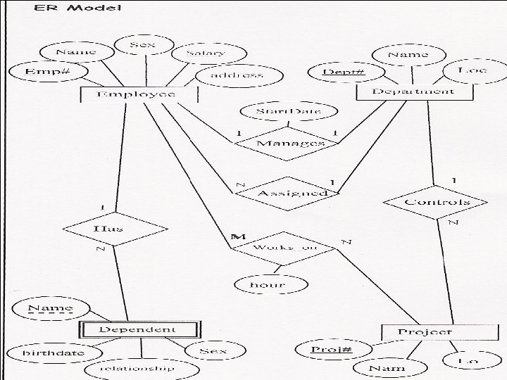
Relational Model for Company Example We will now apply the above rules to the ER Model that we derived for Company example discussed earlier The complete solution is as follows Employee (Emp#, Name, Salary, Address, Sex, Bdate, Dept#, Supervisor. Emp#) Department (Dept#, Name, Mgr. Emp#) Project (Proj#, Name, Sex, Bdate, Relationship) Dependent (Emp#, Name, Sex, Bdate, Relationship)

Relational Model for Company Example Works_On (Emp#, Proj#, Hours, Performance. Rating) Dep_Location ( Dep#, Location) OR+ Employee (Emp#, Name, Salary, Address, Sex, Bdate, Dept#, Mgr. Dept#, Supervisor. Emp#) Department (Dept#, Name)

Summary • Data Modeling – Entity, Attributes and Relationships • Recursive Relationship • Cardinality and Participation • Entity Type – Weak Entity • E/R Model – DBMS Model • Logical Data Model • Relational Data Model – instances, constraints, Keys • Transforming

Data Modeling 3 Ref: A First Course in Database System Jeffrey D Ullman & Jennifer Widom

Is Filing System a Database? Thought Experiment 1: – You and your project partner will be editing the same file. – You both save it at the same time. – Whose changes survive?

Is Filing System a Database? Thought Experiment 2: – You’re updating a file. – The power goes out. – Which of your changes survive?

Advantages of DB over Filing Systems 1. Redundancy can be avoided Name Basic Sal Allowance Desig Accounts Personnel Name Desig Date-of Birth Dep Above two files can be linked on NAME to create a database DESIGN info can then be removed from one of the files

Advantages of DB over Filing Systems 2. Inconsistency can be avoided – direct consequence of previous point.

Advantages of DB over Filing Systems 3. Data independence

Advantages of DB over Filing Systems 4. Efficient data access

Advantages of DB over Filing Systems 5. Sharing of Data allows users to access the same data file at the same Database system has Concurrency Control software for this purpose (This Software uses logical locks)

Advantages of DB over Filing Systems 6. Enforce Security Can be enforce at different levels Database, Record or Tuples, Field Different types of Security - Read and Write - Read - Write - None

Advantages of DB over Filing Systems 7. Enforcing Integrity Constraints Eg. STUDENT Name Course Grade field can be restricted to certain values such as A-E

Advantages of DB over Filing Systems 8. Data administration

Advantages of DB over Filing Systems 9. Concurrent access, crash recovery

Advantages of DB over Filing Systems 10. Up-to-Date information essential for airline reservation systems, banking systems, stork control.

Advantages of DB over Filing Systems 11. Reduced Application Development Time. Two Reasons - Database system has built-in facilities for Concurrency Control, Security and Integrity Enforcement - Database System has a declarative language for programming

So why not use them always? - Expensive/complicated to set up & maintain – This cost & complexity must be offset by need – General-purpose, not suited for special -purpose tasks (e. g. text search!)

Describing Data : Data Model • A data model is a collection of concepts for describing data. • A schema is a description of a particular collection of data, using a given data model. • The relational model of data is the most widely used model today. – Main concept: relation, basically a table with rows and columns. – Every relation has a schema, which describes the columns, or fields.

What’s the intellectual content? • representing information – data modeling • languages and systems for querying data – complex queries with real semantics* – over massive data sets • concurrency control for data manipulation – controlling concurrent access – ensuring transactional semantics • reliable data storage – maintain data semantics even if you pull the plug Syntax : the grammatical correctness - semantics: the meaning or relationship of meanings of a sign or set of signs

OS Support for Data Management • Data can be stored in RAM – this is what every programming language offers! – RAM is fast, and random access • Every OS includes a File System – manages files on a magnetic disk – allows open, read, seek, close on a file – allows protections to be set on a file – drawbacks relative to RAM?

Levels of Abstraction • Views describe how users see the data. • Conceptual schema defines logical structure • Physical schema describes the files and indexes used. • (sometimes called the ANSI/SPARC model) Users View 1 View 2 View 3 Conceptual Schema Physical Schema DB

Examples • Conceptual schema: – Students(sid: string, name: string, login: string, age: integer, gpa: real) – Courses(cid: string, cname: string, credits: integer) – Enrolled(sid: string, cid: string, grade: string) • Physical schema: – Relations stored as unordered files. – Index on first column of Students. • External Schema (View): – Course_info(cid: string, enrollment: integer)

Data Independence Major Objectives of the ANSI Architecture Two major objectives - Logical Data Independence - Physical Data Independence

Data Independence • Logical Data Independence Provide protection from changes in logical structure of data. - provides protection against: - growth eg. Adding a new attribute to a relation restructuring of relations That is, programs which use the data structures need not be modify and re-compiled. The independence is provided by the conceptual / External level Mapping.

Data Independence • Physical Data Independence Protection from changes in physical structure of data. eg. 1 the physical organization of a table changes from sequential to Indexed Sequential - this changes will not require programs that use the database to be modified.

Describing Data ANSI Database Architecture Consists of three levels and two mappings Level 1 Internal Level Contains a schema which describes the file structures that are used to support efficient access to the database. Thus it contains information about the file organization (whether Indexed, Sequential … etc) and also contains information on the sequencing keys, indexed keys, hash keys … etc.

Describing Data Level 2 Conceptual Level Contains a schema that describes the entire database structure in logical terms Thus it will contain all the data types, all the relationships and all the constraints.

Describing Data Level 3 External Level Contains several schema (views), each of which describes a logical subset of the database structure. So a view will contain a description of the part of the database that the particular user is interested in.

Describing Data Mapping 1 Conceptual/ Internal Level Mapping This describes how the internal level is derived from the conceptual level

Describing Data Users View 1 View 2 View 3 Mapping 2 External/ Conceptual Level Mapping Example clustering rows from the DEP and EMP tables into a single file – again no change in programs needed This independence is provided by the Conceptual / Internal level mapping Level 3: External Level Conceptual Schema Physical Schema Level 2: Conceptual Level Mapping 1 Conceptual/ Internal Level Mapping Level 1: Internal Level DB

Database Development Life Cycle. Mini World Requirements Analysis Database Requirements in natural language Conceptual Design Conceptual Schema Data Model Mapping Conceptual schema in DBMS specific terms Physical Database Design Internal Schema

Why is this particularly important for DBMS? • Because rate of change of DB applications is incredibly slow. Discuss!!!.

Concurrency Control • Concurrent execution of user programs: key to good DBMS performance. – Disk accesses frequent, pretty slow – Keep the CPU working on several programs concurrently. • Interleaving actions of different programs: trouble! – e. g. , account-transfer & print statement at same time • DBMS ensures such problems don’t arise. – Users/programmers can pretend they are using a single -user system. (called “Isolation”) – Don’t have to program “very, very carefully”.

Transaction: An Execution of a DB Program • Key concept is a transaction: an atomic sequence of database actions (reads/writes). • Each transaction, executed completely, must take the DB between consistent states. • Users can specify simple integrity constraints on the data. The DBMS enforces these. – Beyond this, the DBMS does not understand the semantics of the data. – Ensuring that a single transaction (run alone) preserves consistency is ultimately the user’s responsibility! Atom : smallest particle of a chemical change

Scheduling Concurrent Transactions • DBMS ensures that execution of {T 1, . . . , Tn} is equivalent to some serial execution T 1’. . . Tn’. – Before reading/writing an object, a transaction requests a lock on the object, and waits till the DBMS gives it the lock. All locks are held until the end of the transaction. (Strict 2 PL locking protocol. ) – Idea: If an action of Ti (say, writing X) affects Tj (which perhaps reads X), … say Ti obtains the lock on X first … so Tj is forced to wait until Ti completes. This effectively orders the transactions. – What if … Tj already has a lock on Y … and Ti later requests a lock on Y? (Deadlock!) Ti or Tj is aborted and restarted!

Ensuring Transaction Properites • DBMS ensures atomicity (all-or-nothing property) even if system crashes in the middle of a Xact. • DBMS ensures durability of committed Xacts even if system crashes. • Idea: Keep a log (history) of all actions carried out by the DBMS while executing a set of Xacts: – Before a change is made to the database, the corresponding log entry is forced to a safe location. (WAL protocol; OS support for this is often inadequate. ) – After a crash, the effects of partially executed transactions are undone using the log. Effects of committed transactions are redone using the log. – trickier than it sounds!

The Log • The following actions are recorded in the log: – Ti writes an object: the old value and the new value. • Log record must go to disk before the changed page! – Ti commits/aborts: a log record indicating this action. • Log records chained together by Xact id, so it’s easy to undo a specific Xact (e. g. , to resolve a deadlock). • Log is often duplexed and archived on “stable” storage. • All log related activities (and in fact, all CC related activities such as lock/unlock, dealing with deadlocks etc. ) are handled transparently by the DBMS.

Structure of a DBMS • A typical DBMS has a layered architecture. • The figure does not show the concurrency control and recovery components. • Each system has its own variations. • The book shows a somewhat more detailed version. These layers must consider concurrency control and recovery Query Optimization and Execution Relational Operators Files and Access Methods Buffer Management Disk Space Management DB

Search” vs. Query • “Search” can return only what’s been “stored” E. g. , best match at i. Won, Google, Ask. Jeeves top ten: • Query: can return new structure of data build from the existing data in the database

A text search engine • • • Less “system” than DBMS – Uses OS files for storage – Just one access method – One hardwired query • regardless of search string Typically no concurrency or recovery management – Read-mostly – Batch-loaded, periodically – No updates to recover – OS a reasonable choice Smarts: text tricks – Search string modifier (e. g. “stemming” and synonyms) – Ranking Engine (sorting the output, e. g. by word or document popularity) Search String Modifier Ranking Engine The Query The Access Method } Simple DBMS Buffer Management. OS Disk Space Management DB There may be time to talk about some of these text tricks in this class, but it won’t be a focus.

Summary • • • Is Filing System a Database? Advantages of DB over Filing System Data Model - Describing Data What’s the intellectual content? OS Support for Data Management Levels of Abstraction & Data Independence Database Development Life Cycle Concurrency Control Transaction: Execution, Scheduling, Concurrent, Ensuring Properties • The Log & The Structure of a DBMS • Query and Search engine & text search engine