Evolutionary Computational Inteliigence Lecture 6 a Multimodality

Evolutionary Computational Inteliigence Lecture 6 a: Multimodality

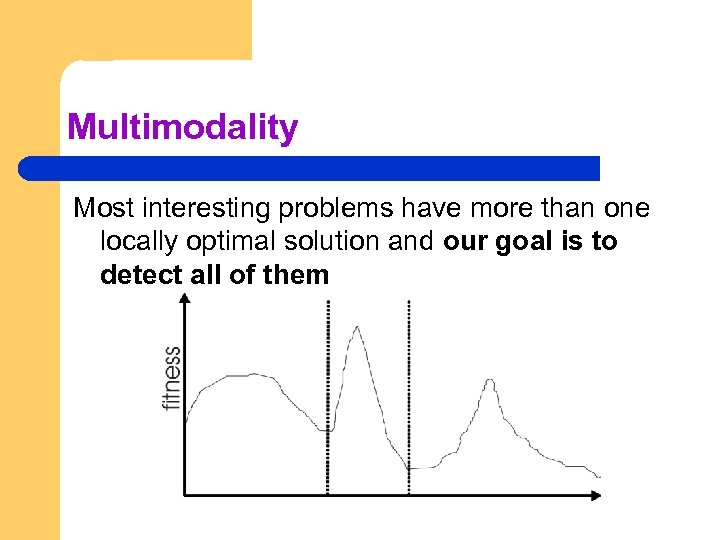Multimodality Most interesting problems have more than one locally optimal solution and our goal is to detect all of them

Multi-Objective Problems (MOPs) l Wide range of problems can be categorised by the presence of a number of n possibly conflicting objectives: – l buying a car: speed vs. price vs. reliability Two part problem: – – finding set of good solutions choice of best for particular application

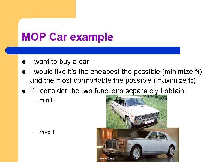MOP Car example l l l I want to buy a car I would like it’s the cheapest the possible (minimize f 1) and the most comfortable the possible (maximize f 2) If I consider the two functions separately I obtain: – min f 1 – max f 2

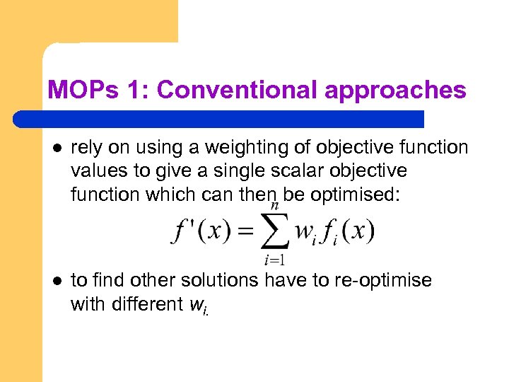MOPs 1: Conventional approaches l rely on using a weighting of objective function values to give a single scalar objective function which can then be optimised: l to find other solutions have to re-optimise with different wi.

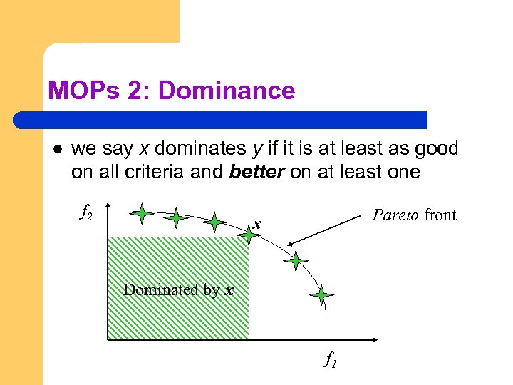MOPs 2: Dominance l we say x dominates y if it is at least as good on all criteria and better on at least one f 2 Pareto front x Dominated by x f 1

Implications for Evolutionary Optimisation l Two main approaches to diversity maintenance: l Implicit approaches (decision space): – – l Impose an equivalent of geographical separation Impose an equivalent of speciation Explicit approaches (fitness): – – Make similar individuals compete for resources (fitness) Make similar individuals compete with each other for survival

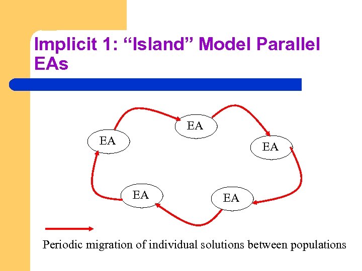Implicit 1: “Island” Model Parallel EAs EA EA EA Periodic migration of individual solutions between populations

Island Model EAs: l l Run multiple populations in parallel, in some kind of communication structure (usually a ring or a torus). After a (usually fixed) number of generations (an Epoch), exchange individuals with neighbours Repeat until ending criteria met Partially inspired by parallel/clustered systems

Island Model Parameter Setting l l The idea is simple but its success is subject to a proper parameter setting It must be somehow known the number of “islands”, i. e. basins of attraction we are considering It must be set the population size for each separate island If some a priori information regarding the fitness landscape is given, island model can be efficient, otherwise it can likely fail

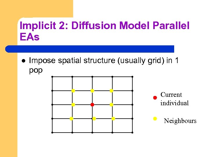Implicit 2: Diffusion Model Parallel EAs l Impose spatial structure (usually grid) in 1 pop Current individual Neighbours

Diffusion Model EAs l l l Consider each individual to exist on a point on a grid Selection (hence recombination) and replacement happen using concept of a neighbourhood a. k. a. deme Leads to different parts of grid searching different parts of space, good solutions diffuse across grid over a number of gens

Diffusion Model Example l l l Assume rectangular grid so each individual has 8 immediate neighbours For each point we can consider a population mad up of 9 individuals One of the other 8 remaining point is selected (e. g. by means of roulette wheel) Recombination between starting and selected point occurs In a steady state logic replacement of the fittest occurs

Implicit 3: Automatic Speciation l l It restricts the recombination on the basis genotypic structure of the solutions in order to have recombination only amongst individual of the same specie – comparing the maximum genotypic distance between solutions – Adding a “tag” (genotypic enlargement) in order to characterize the belonging of each individual to a certain specie In both cases, problem requires a lot of comparisons and the computational overhead can be very high

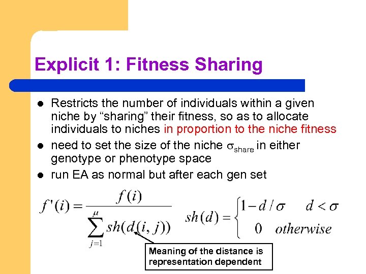Explicit 1: Fitness Sharing l l l Restricts the number of individuals within a given niche by “sharing” their fitness, so as to allocate individuals to niches in proportion to the niche fitness need to set the size of the niche share in either genotype or phenotype space run EA as normal but after each gen set Meaning of the distance is representation dependent

Explicit 2: Crowding l l Attempts to distribute individuals evenly amongst niches relies on the assumption that offspring will tend to be close to parents randomly selects a couple of parents, produce 2 offspring each offspring compete in a pair-tournament for surviving with the most similar parent (steady state) i. e. the parent which has minimal distance

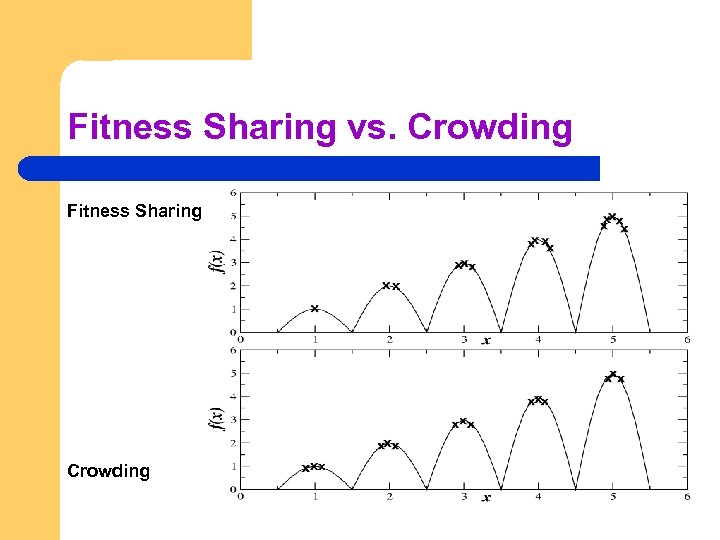Fitness Sharing vs. Crowding Fitness Sharing Crowding

Multimodality and Constraints l l l In some cases we are not satisfied by finding all the local optima but only a subset of them having certain properties (e. g. fitness values) In such cases the combination of algorithmic components can be beneficial A rather efficient and simple option is to properly combine a cascade

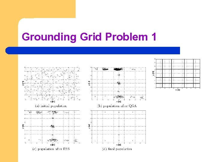
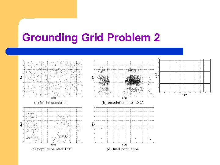
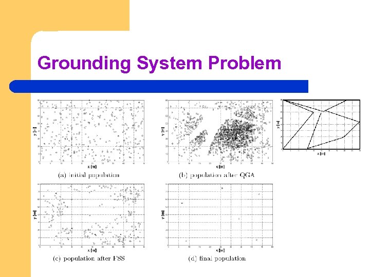
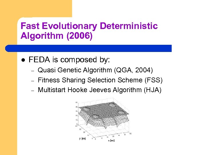Fast Evolutionary Deterministic Algorithm (2006) l FEDA is composed by: – – – Quasi Genetic Algorithm (QGA, 2004) Fitness Sharing Selection Scheme (FSS) Multistart Hooke Jeeves Algorithm (HJA)

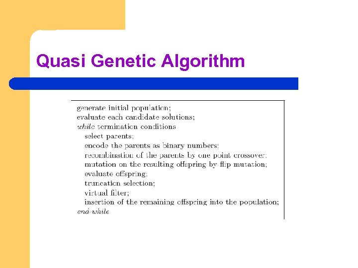Quasi Genetic Algorithm

FEDA l l l The set of solutions coming from QGA (usually a lot) are processed by FSS We thus obtain a smaller set of points which have good fitness values and are spread out in the decision space The HJA is then applied to each of those solutions

Grounding Grid Problem 1

Grounding Grid Problem 2

Grounding System Problem

Evolutionary Computational Inteliigence Lecture 6 b: Towards Parameter Control

Motivation 1 An EA has many strategy parameters, e. g. l mutation operator and mutation rate l crossover operator and crossover rate l selection mechanism and selective pressure (e. g. tournament size) l population size Good parameter values facilitate good performance Q 1 How to find good parameter values ?

Motivation 2 EA parameters are rigid (constant during a run) BUT an EA is a dynamic, adaptive process THUS optimal parameter values may vary during a run Q 2: How to vary parameter values?

Parameter tuning: the traditional way of testing and comparing different values before the “real” run Problems: l users mistakes in settings can be sources of errors or sub-optimal performance l costs much time l parameters interact: exhaustive search is not practicable l good values may become bad during the run (e. g. Population size)

Parameter Setting: Problems l l A wrong parameter setting can lead to an undesirable algorithmic behavious since it can lead to stagnation or premature convergence Too large population size, stagnation Too small population size, premature convergence In some “moments” of the evolution I would like to have a large pop size (when I need to explore and prevent premature convergence); in other “moments” I would like to have a small one (when I need to exploit available genotypes)

Parameter control: setting values on-line, during the actual run, I would like that the algorithm “decides” by itself how to properly vary parameter setting over the run Some popular options for pursuing this aim are: l l l predetermined time-varying schedule p = p(t) using feedback from the search process encoding parameters in chromosomes and rely on natural selection (similar to ES self-adaptation)

Related Problems: l l l finding optimal p is hard, finding optimal p(t) is harder still user-defined feedback mechanism, how to ”optimize”? when would natural selection work for strategy parameters? Provisional answer: l In agreement with the No Free Lunch Theorem, optimal control strategy does not exist. Nevertheless, there a plenty of interesting proposals that can be very performing in some problems. Some of these strategies are very problem oriented while some others are much more robust and thus applicable in a fairly wide spectrum of optimization problems