Evolution of Convolutional Neural Networks Michael Klachko Strukov s

Evolution of Convolutional Neural Networks Michael Klachko Strukov’s Research Group UCSB

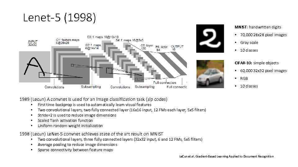Lenet-5 (1998) MNIST: handwritten digits • 70, 000 28 x 28 pixel images • Gray scale • 10 classes CIFAR-10: simple objects • 60, 000 32 x 32 pixel images • RGB • 10 classes 1989 (Lecun) A convnet is used for an image classification task (zip codes) • • • First time backprop is used to automatically learn visual features Two convolutional layers, two fully connected layer (16 x 16 input, 12 FMs each layer, 5 x 5 filters) Stride=2 is used to reduce image dimensions Scaled Tanh activation function Uniform random weight initialization 1998 (Lecun) Le. Net-5 convnet achieves state of the art result on MNIST • • • Two convolutional layers, three fully connected layers (32 x 32 input, 6 and 12 FMs, 5 x 5 filters) Average pooling to reduce image dimensions Sparse connectivity between feature maps Le. Cun et al, Gradient-Based Learning Applied to Document Recognition

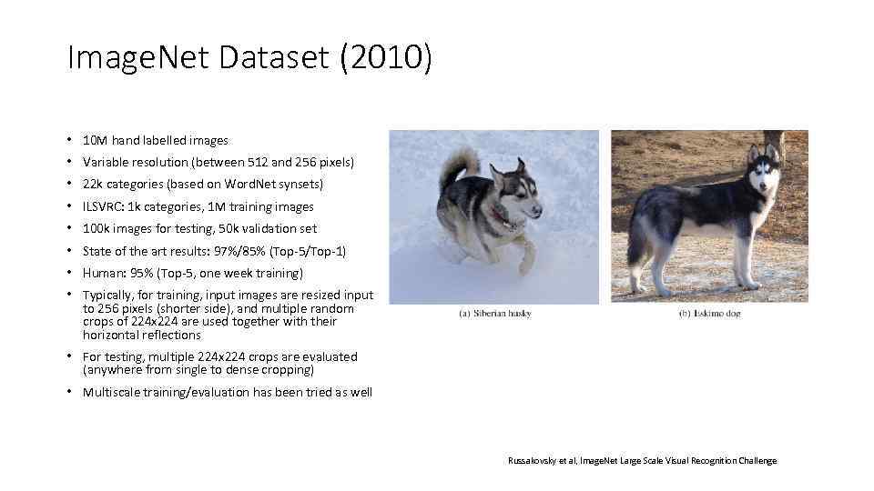Image. Net Dataset (2010) • 10 M hand labelled images • Variable resolution (between 512 and 256 pixels) • 22 k categories (based on Word. Net synsets) • ILSVRC: 1 k categories, 1 M training images • 100 k images for testing, 50 k validation set • State of the art results: 97%/85% (Top-5/Top-1) • Human: 95% (Top-5, one week training) • Typically, for training, input images are resized input to 256 pixels (shorter side), and multiple random crops of 224 x 224 are used together with their horizontal reflections • For testing, multiple 224 x 224 crops are evaluated (anywhere from single to dense cropping) • Multiscale training/evaluation has been tried as well Russakovsky et al, Image. Net Large Scale Visual Recognition Challenge

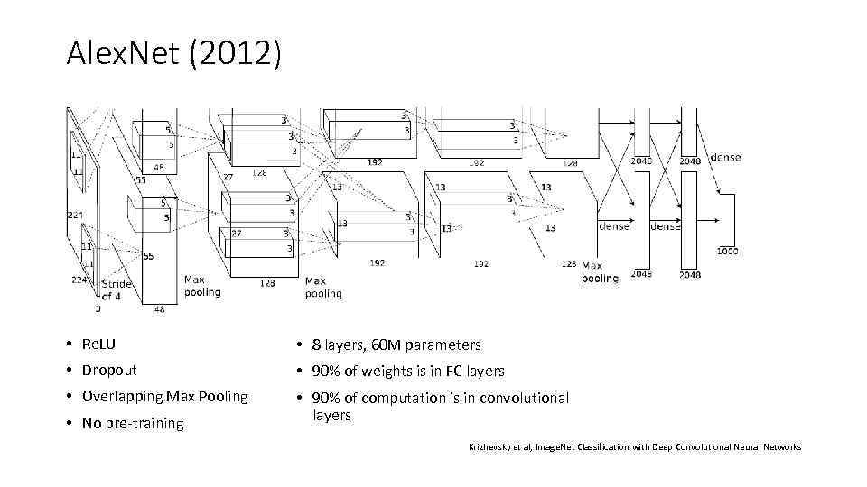Alex. Net (2012) • Re. LU • 8 layers, 60 M parameters • Dropout • 90% of weights is in FC layers • Overlapping Max Pooling • 90% of computation is in convolutional layers • No pre-training Krizhevsky et al, Image. Net Classification with Deep Convolutional Neural Networks

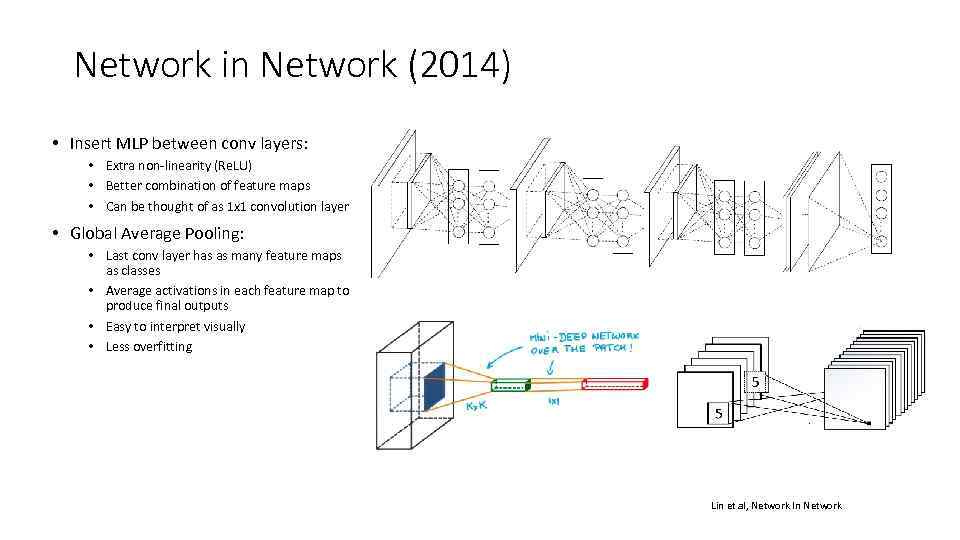Network in Network (2014) • Insert MLP between conv layers: • Extra non-linearity (Re. LU) • Better combination of feature maps • Can be thought of as 1 x 1 convolution layer • Global Average Pooling: • Last conv layer has as many feature maps as classes • Average activations in each feature map to produce final outputs • Easy to interpret visually • Less overfitting Lin et al, Network In Network

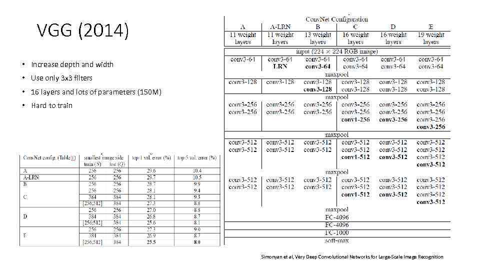VGG (2014) • Increase depth and width • Use only 3 x 3 filters • 16 layers and lots of parameters (150 M) • Hard to train Simonyan et al, Very Deep Convolutional Networks for Large-Scale Image Recognition

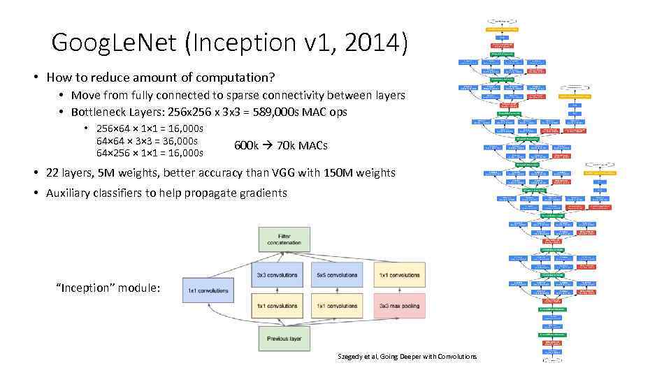Goog. Le. Net (Inception v 1, 2014) • How to reduce amount of computation? • Move from fully connected to sparse connectivity between layers • Bottleneck Layers: 256 x 256 x 3 x 3 = 589, 000 s MAC ops • 256× 64 × 1× 1 = 16, 000 s 64× 64 × 3× 3 = 36, 000 s 64× 256 × 1× 1 = 16, 000 s 600 k 70 k MACs • 22 layers, 5 M weights, better accuracy than VGG with 150 M weights • Auxiliary classifiers to help propagate gradients “Inception” module: Szegedy et al, Going Deeper with Convolutions

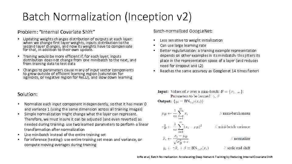Batch Normalization (Inception v 2) Problem: “Internal Covariate Shift” Batch-normalized Goog. Le. Net: • Updating weights changes distribution of outputs at each layer: when we change first layer weights, inputs distribution to the second layer changes, and now its weights have to compensate for that, in addition to their own update. • • Training would be more efficient if, for each layer, inputs distribution does not change from one minibatch to the next, and from training data to test data • Changes to parameters cause many of input vector components to grow outside of efficient learning region (saturation for sigmoids, or negative region for Re. LU), and slow down learning • Less sensitive to weight initialization Can use large learning rate Better regularization: a training example representation depends on other examples in its minibatch: this jitters its place in the representation space of a layer (and reduces need for dropout and L 2) Reaches the same accuracy as Googlenet 14 times faster! Solution: • • Normalize each input component independently, so that it has mean 0 and variance 1 (using the same dimension across all training images) Simple normalization might change what the layer can represent. Therefore, we must insure it can be adjusted (and even reverted) as needed during training: use two learned parameters to perform a linear transformation after normalization Use minibatch instead of the entire training set for inference (testing): use entire training set mean and variance, or compute moving averages during training Ioffe et al, Batch Normalization: Accelerating Deep Network Training by Reducing Internal Covariate Shift

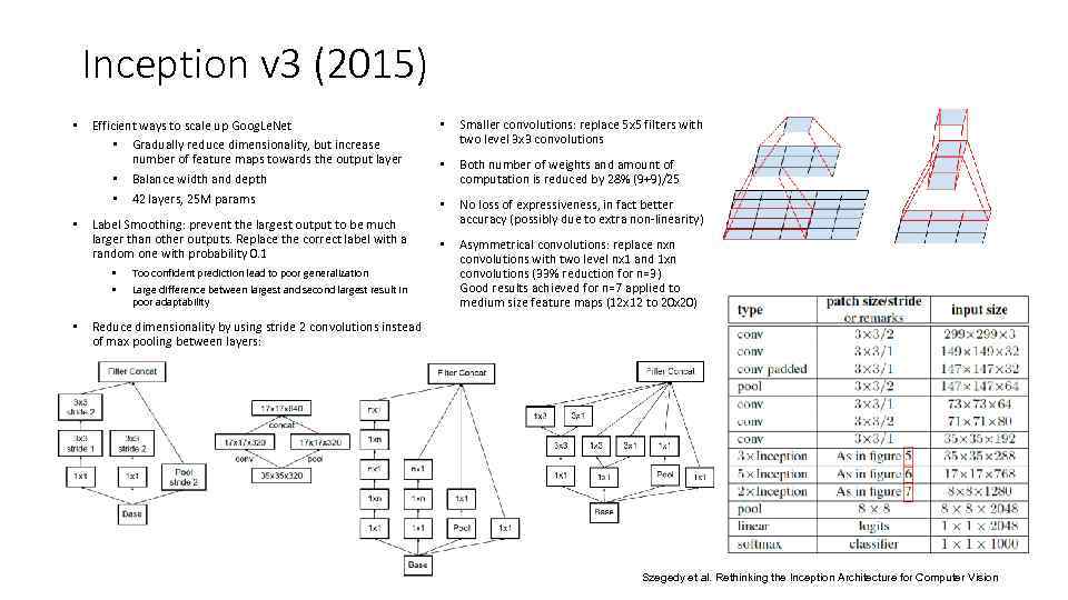Inception v 3 (2015) • • Efficient ways to scale up Goog. Le. Net • Gradually reduce dimensionality, but increase number of feature maps towards the output layer • Balance width and depth • 42 layers, 25 M params Label Smoothing: prevent the largest output to be much larger than other outputs. Replace the correct label with a random one with probability 0. 1 • • • Too confident prediction lead to poor generalization Large difference between largest and second largest result in poor adaptability • Smaller convolutions: replace 5 x 5 filters with two level 3 x 3 convolutions • Both number of weights and amount of computation is reduced by 28% (9+9)/25 • No loss of expressiveness, in fact better accuracy (possibly due to extra non-linearity) • Asymmetrical convolutions: replace nxn convolutions with two level nx 1 and 1 xn convolutions (33% reduction for n=3) Good results achieved for n=7 applied to medium size feature maps (12 x 12 to 20 x 20) Reduce dimensionality by using stride 2 convolutions instead of max pooling between layers: Szegedy et al. Rethinking the Inception Architecture for Computer Vision

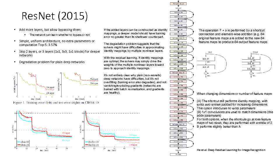Res. Net (2015) • Add more layers, but allow bypassing them: • The network can learn whether to bypass or not • Simple, uniform architecture, no extra parameters or computation Top-5: 3. 57% • Skip 2 layers, or 3 layers (1 x 1, 3 x 3, 1 x 1 blocks) for deeper networks • Degradation problem for plain deep networks If the added layers can be constructed as identity mappings, a deeper model should have training error no greater than its shallower counterpart. The degradation problem suggests that the solvers might have difficulties in approximating identity mappings by multiple nonlinear layers. The operation F + x is performed by a shortcut connection and element-wise addition (e. g. 64 original feature maps are added to the new 64 feature maps to produce 64 output feature maps. With the residual learning, if identity mappings are optimal, the solvers may simply drive the weights of the multiple nonlinear layers toward zero to approach identity mappings. It’s not entirely clear why plain (non-resnets) deep networks have difficulties, but it’s not overfitting (training error also degrades), and not vanishing/exploding gradients (networks are trained with batch normalization, and gradients are healthy). When changing dimensions or number of feature maps: (A) The shortcut still performs identity mapping, with extra zero entries padded for increasing dimensions. This option introduces no extra parameters (B) 1 x 1 convolutions are used to match dimensions (this adds parameters) For both options, when the shortcuts go across feature maps of two sizes, they are performed with a stride of 2. B performs slightly better than A He et al. Deep Residual Learning for Image Recognition

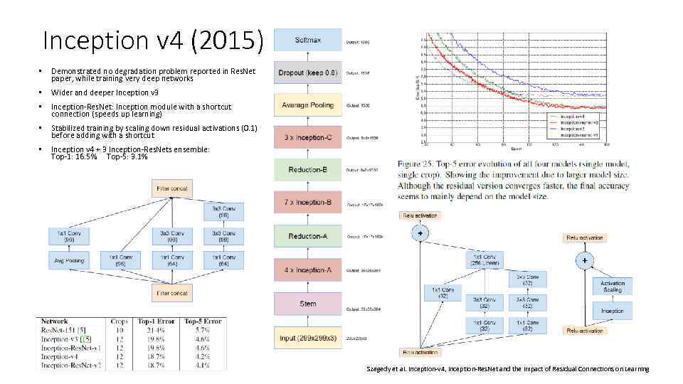Inception v 4 (2015) • Demonstrated no degradation problem reported in Res. Net paper, while training very deep networks • Wider and deeper Inception v 3 • Inception-Res. Net: Inception module with a shortcut connection (speeds up learning) • Stabilized training by scaling down residual activations (0. 1) before adding with a shortcut • Inception v 4 + 3 Inception-Res. Nets ensemble: Top-1: 16. 5% Top-5: 3. 1% Szegedy et al. Inception-v 4, Inception-Res. Net and the Impact of Residual Connections on Learning

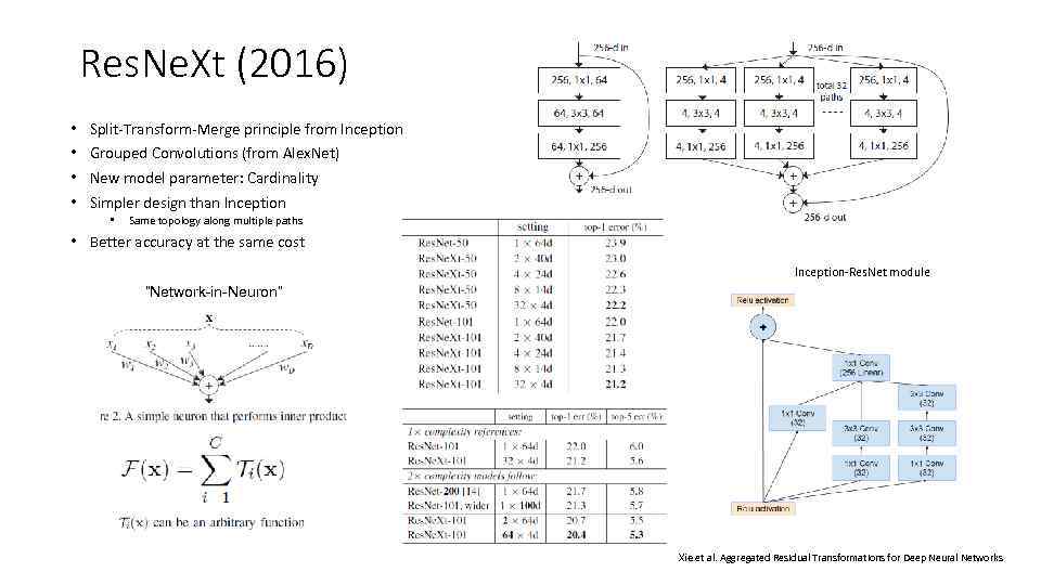Res. Ne. Xt (2016) • • Split-Transform-Merge principle from Inception Grouped Convolutions (from Alex. Net) New model parameter: Cardinality Simpler design than Inception • Same topology along multiple paths • Better accuracy at the same cost Inception-Res. Net module “Network-in-Neuron” Xie et al. Aggregated Residual Transformations for Deep Neural Networks

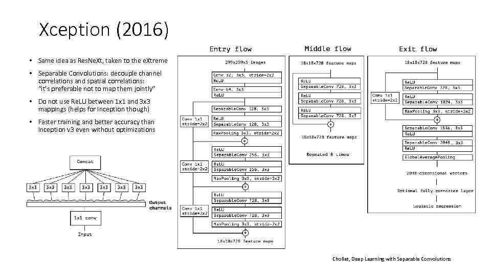Xception (2016) • Same idea as Res. Ne. Xt, taken to the e. Xtreme • Separable Convolutions: decouple channel correlations and spatial correlations: “it’s preferable not to map them jointly” • Do not use Re. LU between 1 х1 and 3 x 3 mappings (helps for Inception though) • Faster training and better accuracy than Inception v 3 even without optimizations Chollet, Deep Learning with Separable Convolutions

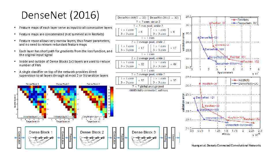Dense. Net (2016) • Feature maps of each layer serve as input to all consecutive layers • Feature maps are concatenated (not summed as in Res. Nets) • Feature reuse allows very narrow layers, thus fewer parameters, and no need to relearn redundant feature maps • Each layer has short path for gradients from the loss function, and the original input signal • Inside and outside of Dense Blocks 1 x 1 layers are used to reduce number of FMs • A single classifier on top of the network provides direct supervision to all layers through at most 2 or 3 transition layers Huang et al, Densely Connected Convolutional Networks

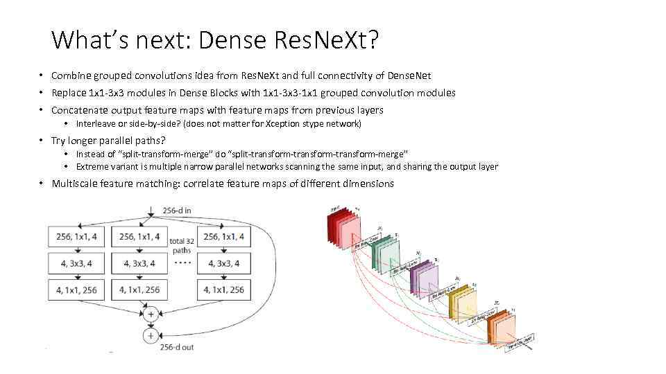What’s next: Dense Res. Ne. Xt? • Combine grouped convolutions idea from Res. Ne. Xt and full connectivity of Dense. Net • Replace 1 x 1 -3 x 3 modules in Dense Blocks with 1 x 1 -3 x 3 -1 x 1 grouped convolution modules • Concatenate output feature maps with feature maps from previous layers • Interleave or side-by-side? (does not matter for Xception stype network) • Try longer parallel paths? • Instead of “split-transform-merge” do “split-transform-transform-merge” • Extreme variant is multiple narrow parallel networks scanning the same input, and sharing the output layer • Multiscale feature matching: correlate feature maps of different dimensions

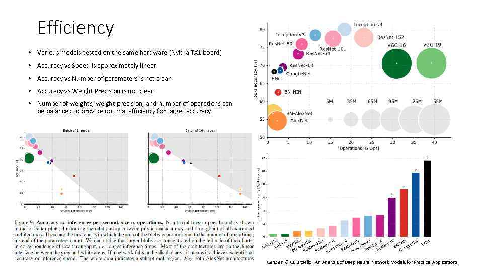Efficiency • Various models tested on the same hardware (Nvidia TX 1 board) • Accuracy vs Speed is approximately linear • Accuracy vs Number of parameters is not clear • Accuracy vs Weight Precision is not clear • Number of weights, weight precision, and number of operations can be balanced to provide optimal efficiency for target accuracy Canziani & Culurciello, An Analysis of Deep Neural Network Models for Practical Applications