6bc4df74d9fa78e41ffb10e146692cf1.ppt
- Количество слайдов: 49
Evaluation and Credibility How much should we believe in what was learned?

Outline § Introduction § Classification with Train, Test, and Validation sets § Handling Unbalanced Data; Parameter Tuning § Cross-validation § Comparing Data Mining Schemes 2
Introduction § How predictive is the model we learned? § Error on the training data is not a good indicator of performance on future data § Q: Why? § A: Because new data will probably not be exactly the same as the training data! § Overfitting – fitting the training data too precisely - usually leads to poor results on new data 3
Evaluation issues § Possible evaluation measures: § Classification Accuracy § Total cost/benefit – when different errors involve different costs § Lift and ROC curves § Error in numeric predictions § How reliable are the predicted results ? 4
Classifier error rate § Natural performance measure for classification problems: error rate § Success: instance’s class is predicted correctly § Error: instance’s class is predicted incorrectly § Error rate: proportion of errors made over the whole set of instances § Training set error rate (resubstitution error) § is way too optimistic! § you can find patterns even in random data 5
Evaluation on “LARGE” data, 1 If many (thousands) of examples are available, including several hundred examples from each class, then how can we evaluate our classifier method? 6
Evaluation on “LARGE” data, 2 § A simple evaluation is sufficient § Randomly split data into training and test sets (usually 2/3 for train, 1/3 for test) § Build a classifier using the train set and evaluate it using the test set. 7
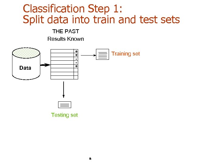
Classification Step 1: Split data into train and test sets THE PAST Results Known Data + + + Training set Testing set 8
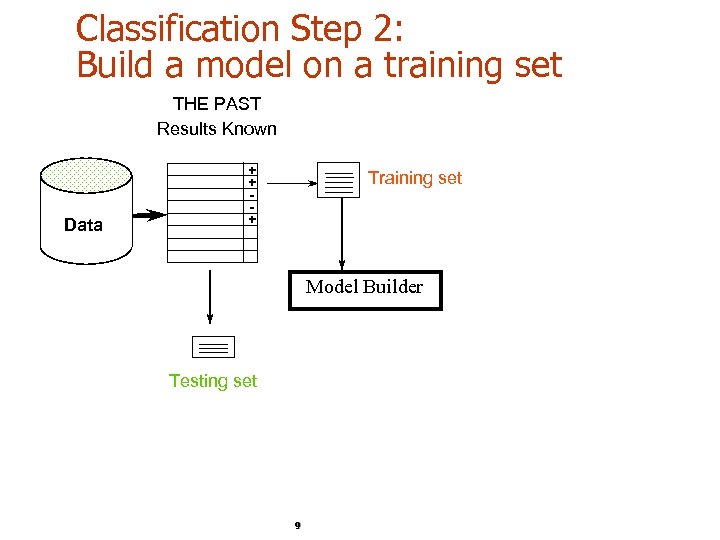
Classification Step 2: Build a model on a training set THE PAST Results Known Data + + + Training set Model Builder Testing set 9
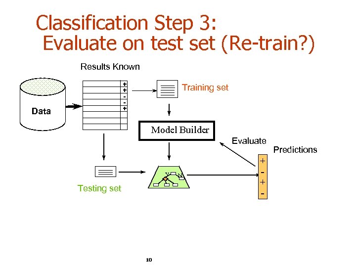
Classification Step 3: Evaluate on test set (Re-train? ) Results Known + + + Data Training set Model Builder Evaluate Y Testing set 10 N + + - Predictions
Unbalanced data § Sometimes, classes have very unequal frequency § Attrition prediction: 97% stay, 3% attrite (in a month) § medical diagnosis: 90% healthy, 10% disease § e. Commerce: 99% don’t buy, 1% buy § Security: >99. 99% of Americans are not terrorists § Similar situation with multiple classes § Majority classifier can be 97% correct, but useless 11
Handling unbalanced data – how? If we have two classes that are very unbalanced, then how can we evaluate our classifier method? 12
Balancing unbalanced data, 1 § With two classes, a good approach is to build BALANCED train and test sets, and train model on a balanced set § randomly select desired number of minority class instances § add equal number of randomly selected majority class § How do we generalize “balancing” to multiple classes? 13
Balancing unbalanced data, 2 § Generalize “balancing” to multiple classes § Ensure that each class is represented with approximately equal proportions in train and test 14

A note on parameter tuning § It is important that the test data is not used in any way to create the classifier § Some learning schemes operate in two stages: § Stage 1: builds the basic structure § Stage 2: optimizes parameter settings § The test data can’t be used for parameter tuning! § Proper procedure uses three sets: training data, validation data, and test data § Validation data is used to optimize parameters witten & eibe 15
Making the most of the data § Once evaluation is complete, all the data can be used to build the final classifier § Generally, the larger the training data the better the classifier (but returns diminish) § The larger the test data the more accurate the error estimate witten & eibe 16
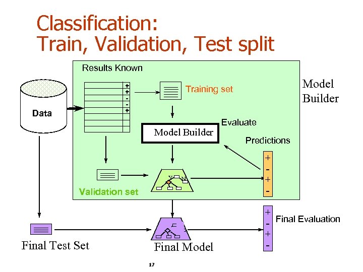
Classification: Train, Validation, Test split Results Known + + + Data Model Builder Y N Validation set Final Test Set Model Builder Training set Final Model 17 Evaluate Predictions + + + - Final Evaluation + -
*Predicting performance § Assume the estimated error rate is 25%. How close is this to the true error rate? § Depends on the amount of test data § Prediction is just like tossing a biased (!) coin § “Head” is a “success”, “tail” is an “error” § In statistics, a succession of independent events like this is called a Bernoulli process § Statistical theory provides us with confidence intervals for the true underlying proportion! witten & eibe 18
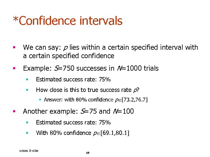
*Confidence intervals § We can say: p lies within a certain specified interval with a certain specified confidence § Example: S=750 successes in N=1000 trials § Estimated success rate: 75% § How close is this to true success rate p? § Answer: with 80% confidence p [73. 2, 76. 7] § Another example: S=75 and N=100 § Estimated success rate: 75% § With 80% confidence p [69. 1, 80. 1] witten & eibe 19
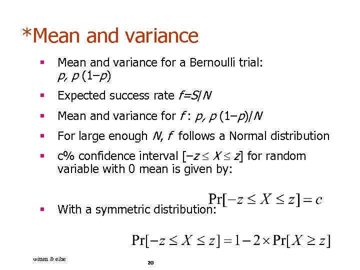
*Mean and variance § Mean and variance for a Bernoulli trial: p, p (1–p) § Expected success rate f=S/N § Mean and variance for f : p, p (1–p)/N § For large enough N, f follows a Normal distribution § c% confidence interval [–z X z] for random variable with 0 mean is given by: § With a symmetric distribution: witten & eibe 20
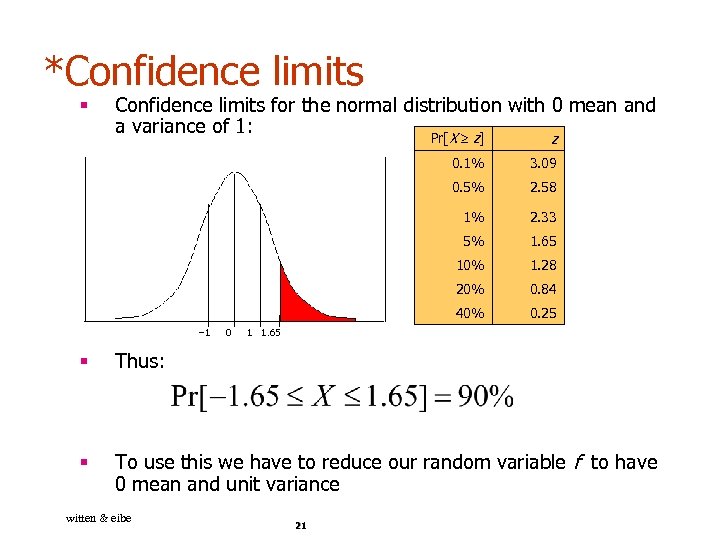
*Confidence limits § Confidence limits for the normal distribution with 0 mean and a variance of 1: Pr[X z] 0. 1% 2. 58 1% 2. 33 5% 1. 65 10% 1. 28 20% 0. 84 40% 0 3. 09 0. 5% – 1 z 0. 25 1 1. 65 § Thus: § To use this we have to reduce our random variable f to have 0 mean and unit variance witten & eibe 21
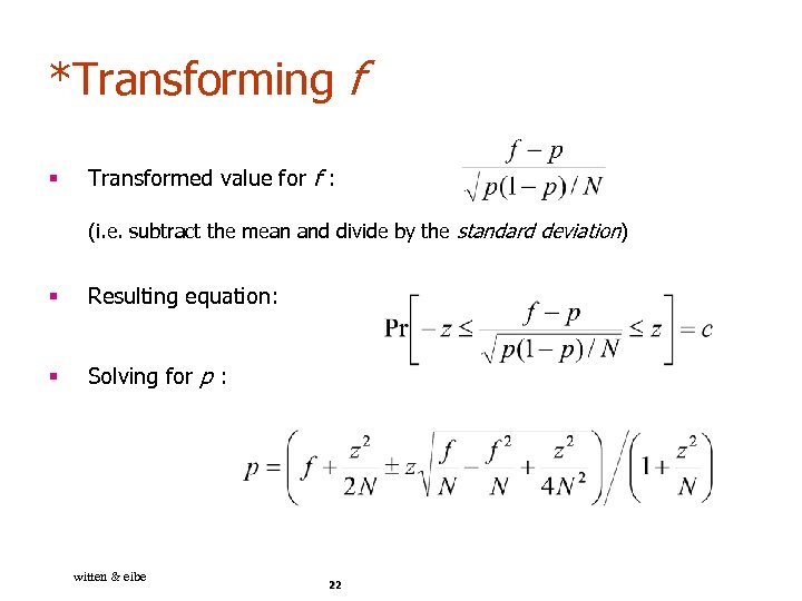
*Transforming f § Transformed value for f : (i. e. subtract the mean and divide by the standard deviation) § Resulting equation: § Solving for p : witten & eibe 22
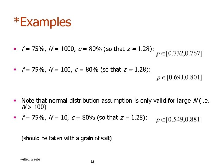
*Examples § f = 75%, N = 1000, c = 80% (so that z = 1. 28): § f = 75%, N = 100, c = 80% (so that z = 1. 28): § Note that normal distribution assumption is only valid for large N (i. e. N > 100) § f = 75%, N = 10, c = 80% (so that z = 1. 28): (should be taken with a grain of salt) witten & eibe 23
Evaluation on “small” data, 1 § The holdout method reserves a certain amount for testing and uses the remainder for training § Usually: one third for testing, the rest for training § For “unbalanced” datasets, samples might not be representative § Few or none instances of some classes § Stratified sample: advanced version of balancing the data § Make sure that each class is represented with approximately equal proportions in both subsets 24
Evaluation on “small” data, 2 § What if we have a small data set? § The chosen 2/3 for training may not be representative. § The chosen 1/3 for testing may not be representative. 25
Repeated holdout method, 1 § Holdout estimate can be made more reliable by repeating the process with different subsamples § In each iteration, a certain proportion is randomly selected for training (possibly with stratification) § The error rates on the different iterations are averaged to yield an overall error rate § This is called the repeated holdout method witten & eibe 26
Repeated holdout method, 2 § Still not optimum: the different test sets overlap. § Can we prevent overlapping? witten & eibe 27
Cross-validation § Cross-validation avoids overlapping test sets § First step: data is split into k subsets of equal size § Second step: each subset in turn is used for testing and the remainder for training § This is called k-fold cross-validation § Often the subsets are stratified before the crossvalidation is performed § The error estimates are averaged to yield an overall error estimate witten & eibe 28
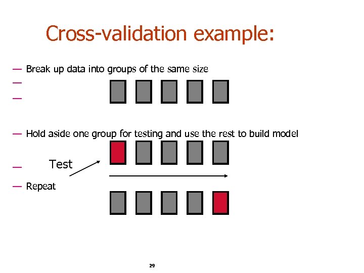
Cross-validation example: — Break up data into groups of the same size — — — Hold aside one group for testing and use the rest to build model — Test — Repeat 29 29
More on cross-validation § Standard method for evaluation: stratified ten-fold cross-validation § Why ten? Extensive experiments have shown that this is the best choice to get an accurate estimate § Stratification reduces the estimate’s variance § Even better: repeated stratified cross-validation § E. g. ten-fold cross-validation is repeated ten times and results are averaged (reduces the variance) witten & eibe 30
Leave-One-Out cross-validation § Leave-One-Out: a particular form of cross-validation: § Set number of folds to number of training instances § I. e. , for n training instances, build classifier n times § Makes best use of the data § Involves no random subsampling § Very computationally expensive § (exception: NN) 31
Leave-One-Out-CV and stratification § Disadvantage of Leave-One-Out-CV: stratification is not possible § § It guarantees a non-stratified sample because there is only one instance in the test set! Extreme example: random dataset split equally into two classes § Best inducer predicts majority class § 50% accuracy on fresh data § Leave-One-Out-CV estimate is 100% error! 32
*The bootstrap § CV uses sampling without replacement § The same instance, once selected, can not be selected again for a particular training/test set § The bootstrap uses sampling with replacement to form the training set § Sample a dataset of n instances n times with replacement to form a new dataset of n instances § Use this data as the training set § Use the instances from the original dataset that don’t occur in the new training set for testing 33
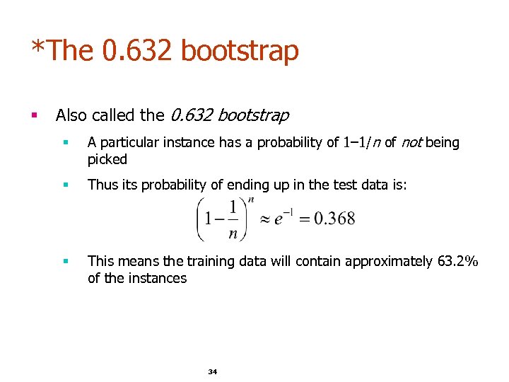
*The 0. 632 bootstrap § Also called the 0. 632 bootstrap § A particular instance has a probability of 1– 1/n of not being picked § Thus its probability of ending up in the test data is: § This means the training data will contain approximately 63. 2% of the instances 34
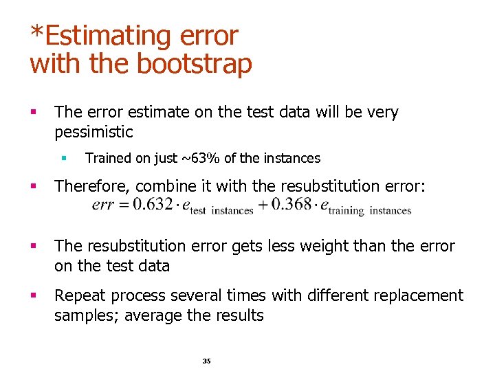
*Estimating error with the bootstrap § The error estimate on the test data will be very pessimistic § Trained on just ~63% of the instances § Therefore, combine it with the resubstitution error: § The resubstitution error gets less weight than the error on the test data § Repeat process several times with different replacement samples; average the results 35
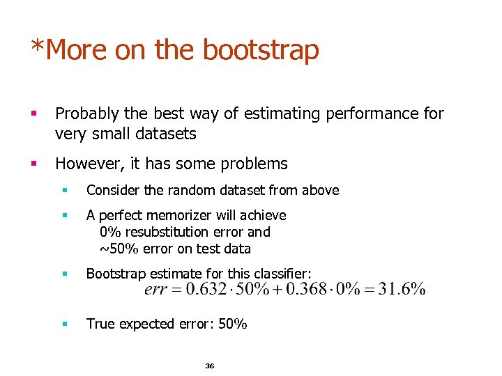
*More on the bootstrap § Probably the best way of estimating performance for very small datasets § However, it has some problems § Consider the random dataset from above § A perfect memorizer will achieve 0% resubstitution error and ~50% error on test data § Bootstrap estimate for this classifier: § True expected error: 50% 36
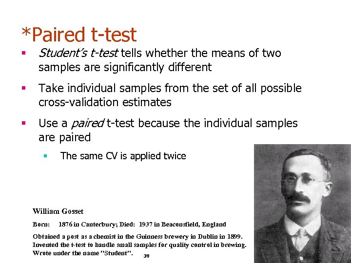
*Paired t-test § Student’s t-test tells whether the means of two § Take individual samples from the set of all possible cross-validation estimates § Use a paired t-test because the individual samples are paired samples are significantly different § The same CV is applied twice William Gosset Born: 1876 in Canterbury; Died: 1937 in Beaconsfield, England Obtained a post as a chemist in the Guinness brewery in Dublin in 1899. Invented the t-test to handle small samples for quality control in brewing. Wrote under the name "Student". 39
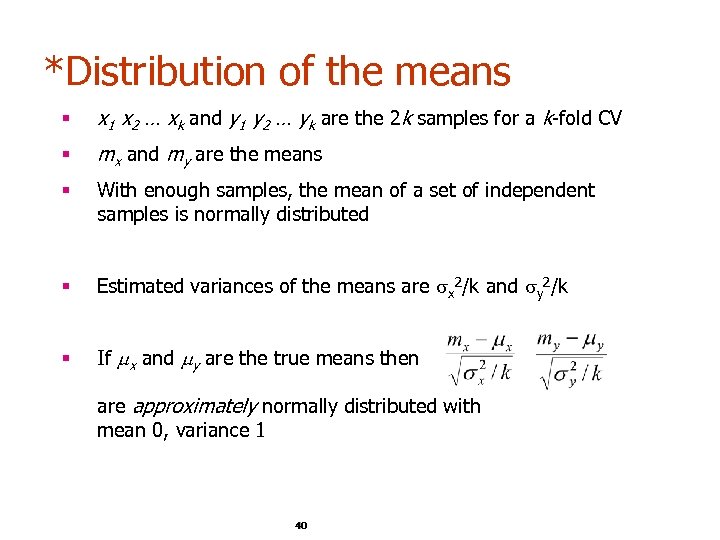
*Distribution of the means § x 1 x 2 … xk and y 1 y 2 … yk are the 2 k samples for a k-fold CV § mx and my are the means § With enough samples, the mean of a set of independent samples is normally distributed § Estimated variances of the means are x 2/k and y 2/k § If x and y are the true means then are approximately normally distributed with mean 0, variance 1 40
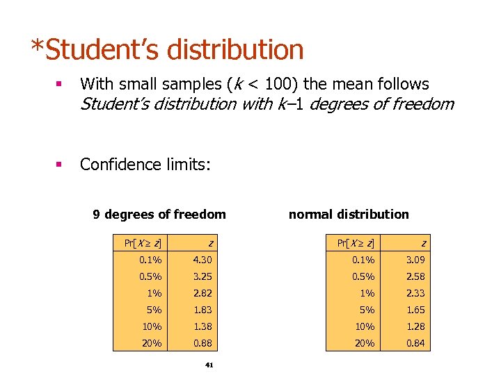
*Student’s distribution § With small samples (k < 100) the mean follows Student’s distribution with k– 1 degrees of freedom § Confidence limits: 9 degrees of freedom normal distribution Pr[X z] z 0. 1% 4. 30 0. 1% 3. 09 0. 5% 3. 25 0. 5% 2. 58 1% 2. 82 1% 2. 33 5% 1. 83 5% 1. 65 10% 1. 38 10% 1. 28 20% 0. 84 41
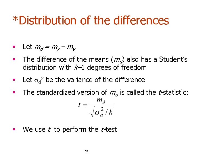
*Distribution of the differences § Let md = mx – my § The difference of the means (md) also has a Student’s distribution with k– 1 degrees of freedom § Let d 2 be the variance of the difference § The standardized version of md is called the t-statistic: § We use t to perform the t-test 42
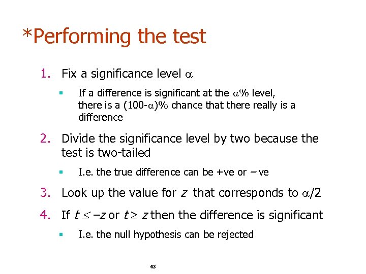
*Performing the test 1. Fix a significance level § If a difference is significant at the % level, there is a (100 - )% chance that there really is a difference 2. Divide the significance level by two because the test is two-tailed § I. e. the true difference can be +ve or – ve 3. Look up the value for z that corresponds to /2 4. If t –z or t z then the difference is significant § I. e. the null hypothesis can be rejected 43
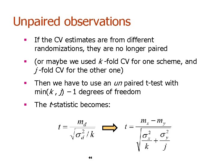
Unpaired observations § If the CV estimates are from different randomizations, they are no longer paired § (or maybe we used k -fold CV for one scheme, and j -fold CV for the other one) § Then we have to use an un paired t-test with min(k , j) – 1 degrees of freedom § The t-statistic becomes: 44
*Interpreting the result § All our cross-validation estimates are based on the same dataset § Hence the test only tells us whether a complete k-fold CV for this dataset would show a difference § § Complete k-fold CV generates all possible partitions of the data into k folds and averages the results Ideally, should use a different dataset sample for each of the k-fold CV estimates used in the test to judge performance across different training sets 45
T-statistic many uses § Looking ahead, we will come back to use of Tstatistic for gene filtering later 46
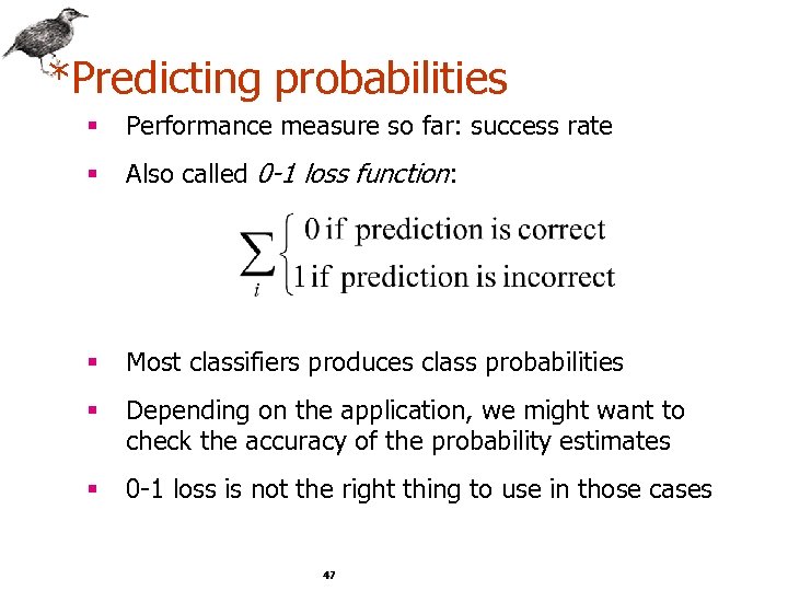
*Predicting probabilities § Performance measure so far: success rate § Also called 0 -1 loss function: § Most classifiers produces class probabilities § Depending on the application, we might want to check the accuracy of the probability estimates § 0 -1 loss is not the right thing to use in those cases 47
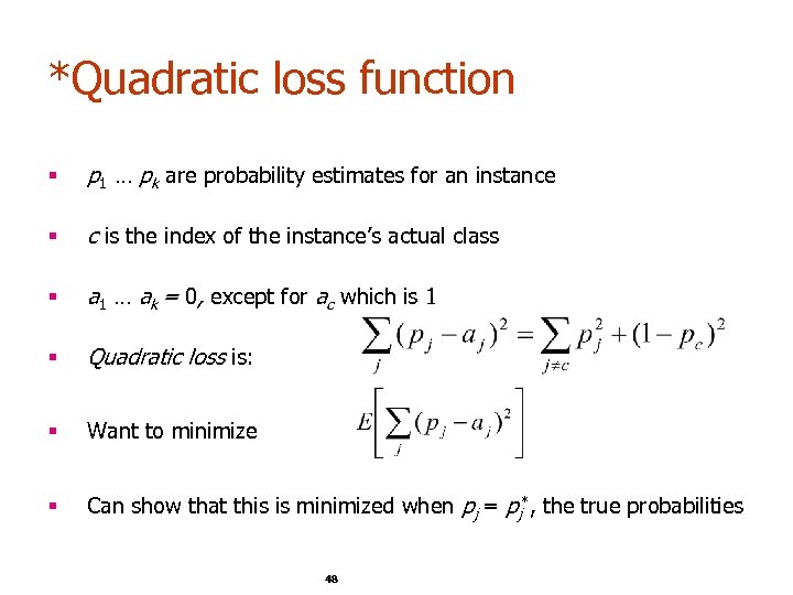
*Quadratic loss function § p 1 … pk are probability estimates for an instance § c is the index of the instance’s actual class § a 1 … ak = 0, except for ac which is 1 § Quadratic loss is: § Want to minimize § Can show that this is minimized when pj = pj*, the true probabilities 48
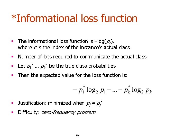
*Informational loss function § The informational loss function is –log(pc), where c is the index of the instance’s actual class § Number of bits required to communicate the actual class § Let p 1* … pk* be the true class probabilities § Then the expected value for the loss function is: § Justification: minimized when pj = pj* § Difficulty: zero-frequency problem 49
*Discussion § Which loss function to choose? § § Quadratic loss function takes into account all class probability estimates for an instance § Informational loss focuses only on the probability estimate for the actual class § Quadratic loss is bounded: § § Both encourage honesty Informational loss can be infinite it can never exceed 2 Informational loss is related to MDL principle 50 [later]
Evaluation Summary: § Use Train, Test, Validation sets for “LARGE” data § Balance “un-balanced” data § Use Cross-validation for small data § Don’t use test data for parameter tuning - use separate validation data § Most Important: Avoid Overfitting 51
6bc4df74d9fa78e41ffb10e146692cf1.ppt