

0f7336f64d048a7f63fbd2c6660b7313.ppt
- Количество слайдов: 51
 ESRC Census Development Programme Identifying the cash-rich and the cash-poor: Lessons from the Census Rehearsal Dr Paul Williamson Department of Geography
 Why is income so important? • Arguably the most direct measure of utility [Yes, I know - “Money can’t buy happiness”] • Helps target Neighbourhood renewal • Helps with planning – [of houses, shops, leisure facilities…] • Consumer marketing • Tax-benefit analysis
 • Most requested addition to 2001 Census
 The 2001 Census Geography of income:
 Other sources of data on income • Benefits data • Government surveys (e. g. GHS, LFS, FES, FRS, NES) • Commercially-held data [Postcode sector and postcode unit estimates] • The Census Rehearsal (1999)
 Key Objectives Evaluation of: • Extant methods for small-area income estimation • New approaches • Utility of non-census information (e. g. council tax; house price; benefits data) [ • Methods of imputing income band means ]
 Definition of ‘income’ • • • Income Wealth Gross or net income? Pre or post housing costs? Adult or Household? – Total – Equivalised [Per capita / OECD / Mc. Clements]
 Surrogates • Univariate – % unemployed – % 2+ car households – % residents in Social Classes I + II – % owner-occupation
 – Carstairs [Unemployment, overcrowding; not owning car; head in") • Multivariate (deprivation indices) – Carstairs [Unemployment, overcrowding; not owning car; head in Social Class IV or V] – Townsend [Unemployment; overcrowding; not owning home; not owning car] – Breadline [not owning car; not owning house; lone parenthood; social class IV or V; illness; unemployment]
• Multivariate (deprivation indices) – Carstairs [Unemployment, overcrowding; not owning car; head in Social Class IV or V] – Townsend [Unemployment; overcrowding; not owning home; not owning car] – Breadline [not owning car; not owning house; lone parenthood; social class IV or V; illness; unemployment]
 [owning 2+ cars; NS-SEC") – DLTR Index of Multiple Deprivation 2000 – Green (Wealth) [owning 2+ cars; NS-SEC I or II; High qualifications]
– DLTR Index of Multiple Deprivation 2000 – Green (Wealth) [owning 2+ cars; NS-SEC I or II; High qualifications]
 • Geodemographic – Super. Profiles – MOSAIC – GB Profiles
![• Model Individual income – Dale (SOC 2000; Economic activity; age; sex; Region]](https://present5.com/presentation/0f7336f64d048a7f63fbd2c6660b7313/image-12.jpg "• Model Individual income – Dale (SOC 2000; Economic activity; age; sex; Region]") • Model Individual income – Dale (SOC 2000; Economic activity; age; sex; Region] – Lee (SOC 2000; Economic activity] – Regression (individual and/or ecological) Household income – Regression (household and/or ecological) – Bramley & Smart (H/h comp. ; earners; tenure; area level deprivation)
• Model Individual income – Dale (SOC 2000; Economic activity; age; sex; Region] – Lee (SOC 2000; Economic activity] – Regression (individual and/or ecological) Household income – Regression (household and/or ecological) – Bramley & Smart (H/h comp. ; earners; tenure; area level deprivation)
 The 1999 Census Rehearsal Key features • full census questionnaire + INCOME • Large achieved sample – c. 65, 000 households – c. 140, 000 individuals • Spatially contiguous
![Clustered sampling strategy: – 7 part districts [Excluding NI] – 38 wards – 650](https://present5.com/presentation/0f7336f64d048a7f63fbd2c6660b7313/image-14.jpg "Clustered sampling strategy: – 7 part districts [Excluding NI] – 38 wards – 650") Clustered sampling strategy: – 7 part districts [Excluding NI] – 38 wards – 650 EDs
Clustered sampling strategy: – 7 part districts [Excluding NI] – 38 wards – 650 EDs
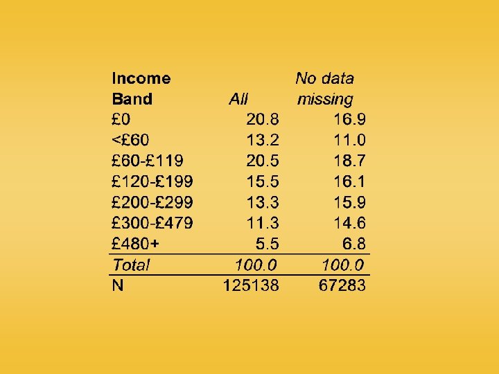
 – income (~15%) – other") Potential problems • non-response rate – overall (~ 50%) – income (~15%) – other variables (5 -20%) – full responses for ~ 55 % of achieved sample [individuals and households] • non-response bias
Potential problems • non-response rate – overall (~ 50%) – income (~15%) – other variables (5 -20%) – full responses for ~ 55 % of achieved sample [individuals and households] • non-response bias

 • Banding of income question What is your total current gross income from all sources? Per week Nil Less than £ 60 to £ 119 £ 120 to £ 199 £ 200 to £ 299 £ 300 to £ 479 £ 480 or more or _ _ _ Per year (approximately) Nil Less than £ 3, 000 _ £ 3, 000 to £ 5, 999 £ 6, 000 to £ 9, 999 £ 10, 000 to £ 14, 999 £ 15, 000 to £ 24, 999 £ 25, 000 or more
 – Only 10% of adults in top band – but problem compounded when individual incomes aggregated to estimate household income – band mid-point band mean – value of band means area sensitive?
") Source: FRS 1998/9 (Crown Copyright)
Source: FRS 1998/9 (Crown Copyright)
 Digression: modelling income band means Alternative modelling strategies include: • National mean • Sub-group mean (e. g. by council tax band) • Statistical distributions (log-normal; pareto) • New variant of log-normal approach with addition of modelled median etc.
 Results • For all bands sub-group mean best – if possible • For closed-bands, national mean is next best • For open (top) band, new proposed lognormal approach is best, particularly where there is evidence of strong spatial clustering
 Results of modelling top income band
 Results of modelling top income band
 • Spatial scale – At what scale does income vary most? • MAUP – 1991 vs 1998/9 boundaries – zones with <10 households or 25 residents excluded from analysis • SOC 2000 / NS-SEC – Lack of alternative SOC 2000 coded data – Therefore have to use Census Rehearsal data – Use partitioned data to avoid unduly advantaging SOC 2000 based approaches
 Results
 Census Rehearsal Income Distribution
 Heterogeneity rules OK! • At ward level the % household reps. in top income-band averaged 9. 1% – but ranged from 2. 8% to 21. 6% • 89% of EDs contained one or more household reps. in top income-band – i. e. in top income-decile of the population

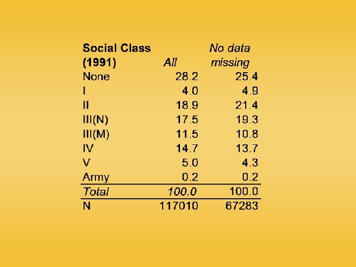
 Missing data • Missing data have minimal impact on results – From ‘Raw’ to ‘Ideal’ data, most correlations change by <0. 02 – Very few values change by >0. 05 – Exception is NS-SEC 8 [by definition!] – Correlations lower for ‘Ideal’ than ‘Raw’ • Surrogates calculated direct from Rehearsal – circumvents data response bias?
 Scale • Higher correlations at higher geographies • District effect small but significant – BUT none of districts in SE England Overfitting • No significant impact
 MAUP • Correlations vary by up to 0. 1 between alternative boundaries at same spatial scale BUT • No detectable effect on rankings of surrogate income measures
") Adult income (r 2)
Adult income (r 2)
 • • Age, Age 2, sex, ethnicity, marital status Type and") Regression model (adults) • • Age, Age 2, sex, ethnicity, marital status Type and tenure of dwelling Qualifications Economic (in)activity and health Mean SOC 2000 and SIC 2000 income Supervisory status District of residence
Regression model (adults) • • Age, Age 2, sex, ethnicity, marital status Type and tenure of dwelling Qualifications Economic (in)activity and health Mean SOC 2000 and SIC 2000 income Supervisory status District of residence
 Caveats • ‘Best’ performing surrogates in danger of over-fitting? – For Dale, Lee and Voas mean occupational income calculated directly from Census Rehearsal dataset (no other SOC 2000 sources available at time of analysis) BUT – No significant difference if SOC minor or unit codes used – No significant difference if data partitioned
") Household income (r 2)
Household income (r 2)
 Accuracy • For many purposes relative, rather than absolute, accuracy is most important ranking


 Other data sources • < 1% of unexplained spatial variation in income attributable to area level effects • House price has no significant impact – could be due to data problems • Council tax band has small but significant effect [for areas of enumeration district size and below] • Lack of utility counter-intuitive? – current value purchase price – purchase income current income
 • Best approaches capture 80 -90% of spatial variation in income, even") Conclusions (I) • Best approaches capture 80 -90% of spatial variation in income, even for smallest spatial units • But considerable within-area heterogeneity • Best approaches are regression or subgroup mean based • Conventional deprivation indices a poor second to % social class / NS-SEC I+II
Conclusions (I) • Best approaches capture 80 -90% of spatial variation in income, even for smallest spatial units • But considerable within-area heterogeneity • Best approaches are regression or subgroup mean based • Conventional deprivation indices a poor second to % social class / NS-SEC I+II
 • Geodemographic classifications at best perform as well as % NS-SEC I+II,") Conclusions (II) • Geodemographic classifications at best perform as well as % NS-SEC I+II, and perform best for areas of ward size and above • Qualified support for use of statistical distributions in modelling top income band means
Conclusions (II) • Geodemographic classifications at best perform as well as % NS-SEC I+II, and perform best for areas of ward size and above • Qualified support for use of statistical distributions in modelling top income band means
 Implications Moral for marketers: • Target people, not places Moral for policy makers: • Deprivation indices not the best proxy for income • ONS ward income estimates (based on ecological regression) likely to perform well
 • Lobby") Longer term • Consider external correlates (e. g. IMD 2000; benefits data) • Lobby for Census Office to create smallarea income estimate – by imputing income on Census microdata – include non-census information (? )
Longer term • Consider external correlates (e. g. IMD 2000; benefits data) • Lobby for Census Office to create smallarea income estimate – by imputing income on Census microdata – include non-census information (? )
 Acknowledgements • House price data were taken from the Experían Limited Postal Sector Data, ESRC/JISC Agreement. • Grateful thanks are due to the Census Custodians of England, Wales and Scotland for granting permission to access the Census Rehearsal dataset. • A debt of gratitude is also owed to a number at the Office for National Statistics, in particular Keith Whitfield and Philip Clarke. • Finally, thanks are due to David Voas for undertaking some of the preparatory work for this project. • All analyses and conclusions remain the sole responsibility of the Dr Paul Williamson.
 • NS-SEC I+II: % persons aged 16 -74 in NS-SEC I or") Definitions (I) • NS-SEC I+II: % persons aged 16 -74 in NS-SEC I or II • Townsend: Multiple deprivation indicator based on % economically active unemployed; % overcrowded households; % households with no car and % of households not owner occupied • Green (Wealth): Affluence indicator based on % households with 2+ cars; % persons aged 16 -74 in NS-SEC I and % adults with high educational qualifications • PCA_96: Geodemographic classification based on principal components analysis of 20 normalised census variables, individuals in each of 96 area types assumed to have mean income of all persons in area type • Voas: Alternative geodemographic classification, in which five census variables are divided into above or below median, one variable into thirds; with all cross-tabulated to give a total of 96 discrete area types
Definitions (I) • NS-SEC I+II: % persons aged 16 -74 in NS-SEC I or II • Townsend: Multiple deprivation indicator based on % economically active unemployed; % overcrowded households; % households with no car and % of households not owner occupied • Green (Wealth): Affluence indicator based on % households with 2+ cars; % persons aged 16 -74 in NS-SEC I and % adults with high educational qualifications • PCA_96: Geodemographic classification based on principal components analysis of 20 normalised census variables, individuals in each of 96 area types assumed to have mean income of all persons in area type • Voas: Alternative geodemographic classification, in which five census variables are divided into above or below median, one variable into thirds; with all cross-tabulated to give a total of 96 discrete area types
 • Dale: Income imputed given mean income for population sub-group defined by") Definitions (II) • Dale: Income imputed given mean income for population sub-group defined by sex, SOC 2000 minor group, economic activity (missing; employed full-time; employed part-time; self-employed; other), age (missing; 0 -15; 16 -19; 20 -29; 30 -49; 50+) [Maximum of 4860 valid sub-groups] • Lee: Income imputed given mean income for population sub-group defined by SOC 2000 minor group, economic activity (child; not applicable; employed full-time; employed part-time; self-employed; unemployed; retired; other inactive) [maximum of 649 valid subgroups]
Definitions (II) • Dale: Income imputed given mean income for population sub-group defined by sex, SOC 2000 minor group, economic activity (missing; employed full-time; employed part-time; self-employed; other), age (missing; 0 -15; 16 -19; 20 -29; 30 -49; 50+) [Maximum of 4860 valid sub-groups] • Lee: Income imputed given mean income for population sub-group defined by SOC 2000 minor group, economic activity (child; not applicable; employed full-time; employed part-time; self-employed; unemployed; retired; other inactive) [maximum of 649 valid subgroups]
 • Voas (individual): Regression model for adult income (children assumed to have") Definitions (III) • Voas (individual): Regression model for adult income (children assumed to have 0 income); INCOME 0. 5 predicted given: mean income by SOC 2000 unit; mean income by Industry category, age 2, residents 2, rooms and cars plus dummy variables for sex, white, full-time student, married, Single/Widowed/Divorced, Longterm ill, No qualifications, GCSE or equivalent, A levels or equivalent, Undergraduate degree or equivalent, employed full-time, employed part-time, self-employed, unemployed, retired, permanently sick, other economically inactive excluding pensioners and students, Semi-detached, terrace, flat, caravan, privately rented, social rented, employed manager or supervisor and district of residence • Voas (household): Regression model for total household income; HHINC 0. 5 predicted given same set of predictors as for Voas (individual), but based only upon head of household’s characteristics
Definitions (III) • Voas (individual): Regression model for adult income (children assumed to have 0 income); INCOME 0. 5 predicted given: mean income by SOC 2000 unit; mean income by Industry category, age 2, residents 2, rooms and cars plus dummy variables for sex, white, full-time student, married, Single/Widowed/Divorced, Longterm ill, No qualifications, GCSE or equivalent, A levels or equivalent, Undergraduate degree or equivalent, employed full-time, employed part-time, self-employed, unemployed, retired, permanently sick, other economically inactive excluding pensioners and students, Semi-detached, terrace, flat, caravan, privately rented, social rented, employed manager or supervisor and district of residence • Voas (household): Regression model for total household income; HHINC 0. 5 predicted given same set of predictors as for Voas (individual), but based only upon head of household’s characteristics