Equity Portfolio Management 02 02 09 Passive versus Active

Equity Portfolio Management 02/02/09

Passive versus Active Management • Passive equity portfolio management • Long-term buy-and-hold strategy • Usually tracks an index over time • Designed to match market performance • Manager is judged on how well they track the target index • Active equity portfolio management • Attempts to outperform a passive benchmark portfolio on a risk-adjusted basis 2

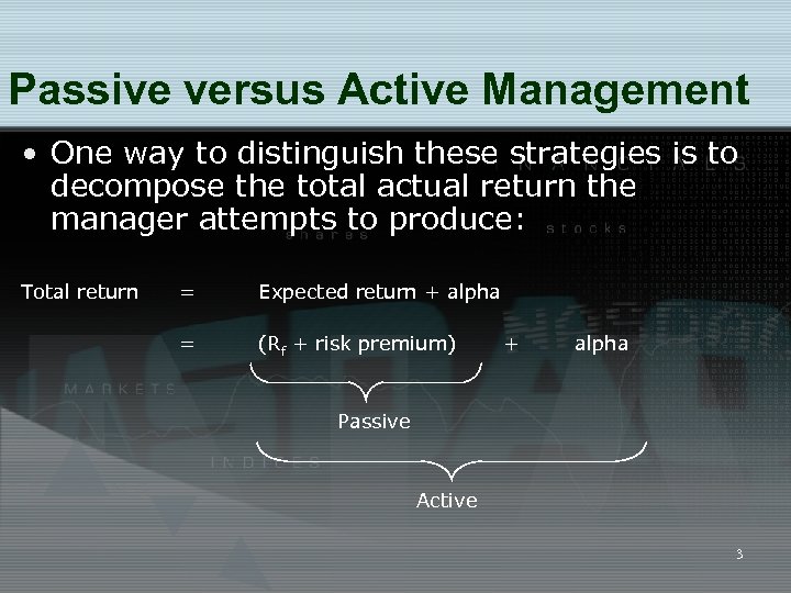Passive versus Active Management • One way to distinguish these strategies is to decompose the total actual return the manager attempts to produce: Total return = Expected return + alpha = (Rf + risk premium) + alpha Passive Active 3

An Overview of Passive Equity Portfolio Management Strategies • Replicate the performance of an index • May slightly underperform the target index due to fees and commissions • Costs of active management (1 to 2 percent) are hard to overcome in risk-adjusted performance 4

Index Portfolio Construction Techniques • Full replication • Sampling • Completeness Funds 5

Full Replication • All securities in the index are purchased in proportion to weights in the index • This helps ensure close tracking • Increases transaction costs, particularly with dividend reinvestment 6

Sampling • Buys a representative sample of stocks in the benchmark index according to their weights in the index • Fewer stocks means lower commissions • Reinvestment of dividends is less difficult • Will not track the index as closely, so there will be some tracking error • Tracking error is the extent to which return fluctuation in the portfolio is not correlated with benchmark return fluctuation. 7

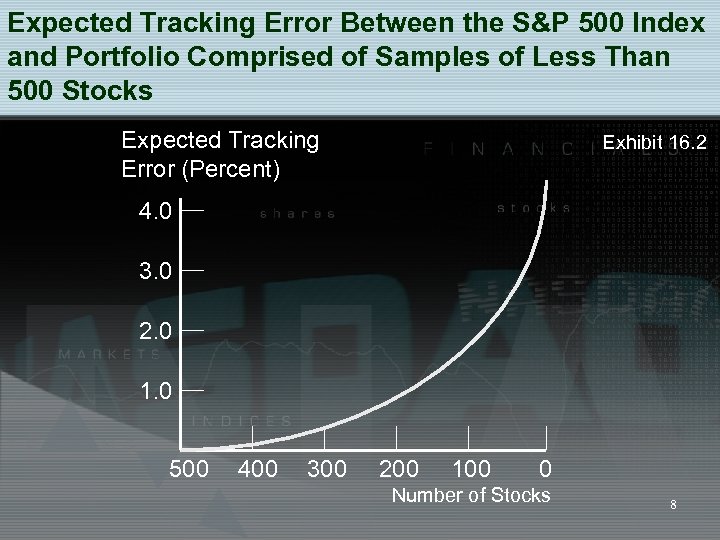Expected Tracking Error Between the S&P 500 Index and Portfolio Comprised of Samples of Less Than 500 Stocks Expected Tracking Error (Percent) Exhibit 16. 2 4. 0 3. 0 2. 0 1. 0 500 400 300 200 100 0 Number of Stocks 8

Calculating Tracking Error • The annualized tracking error for a portfolio is calculated as: where 9

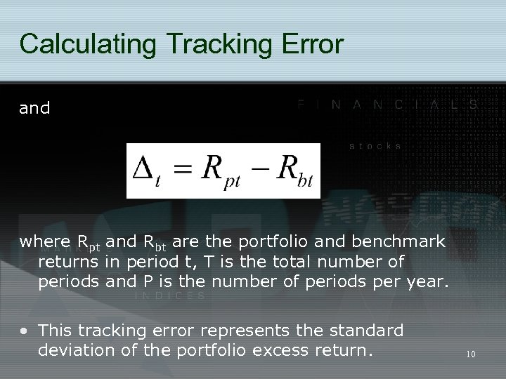Calculating Tracking Error and where Rpt and Rbt are the portfolio and benchmark returns in period t, T is the total number of periods and P is the number of periods per year. • This tracking error represents the standard deviation of the portfolio excess return. 10

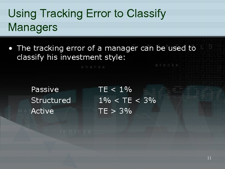Using Tracking Error to Classify Managers • The tracking error of a manager can be used to classify his investment style: Passive Structured Active TE < 1% 1% < TE < 3% TE > 3% 11

Completeness Funds • Completeness funds complement active portfolios. • Funds are allocated to sectors and styles that are not represented in the active portfolios 12

Justification for indexing • Markets are efficient OR • There are superior managers but it is difficult to identify them before the fact OR • The potential for higher returns from active management does not compensate for the higher risk and higher transaction costs 13

Efficient Capital Markets • In an efficient capital market, security prices adjust rapidly to the arrival of new information. • Whether markets are efficient has been extensively researched and remains controversial. 14

Why Should Capital Markets Be Efficient? • The premises of an efficient market • A large number of competing profit-maximizing participants analyze and value securities, each independently of the others • New information regarding securities comes to the market in a random fashion • Profit-maximizing investors adjust security prices rapidly to reflect the effect of new information • Conclusion: In an efficient market, the expected returns implicit in the current price 15 of a security should reflect its risk

Efficient Market Hypotheses (EMH) • Weak-Form EMH - prices reflect all security-market information • Semistrong-form EMH - prices reflect all public information • Strong-form EMH - prices reflect all public and private information 16

Weak-Form EMH • Current prices reflect all securitymarket information, including the historical sequence of prices, rates of return, trading volume data, and other market-generated information. • Implication (i. e. , if hypothesis holds): Past rates of return and other market data should have no relationship with future rates of return. 17

Weak-Form EMH • Tests: Runs tests, filter rule tests • Results: Results generally support the weak-form EMH, but results are not unanimous 18

Semistrong-Form EMH • Current security prices reflect all public information, such as firm and market related announcements, P/E ratios, P/BV ratios, etc. • Implication: Decisions made on new information after it is public should not lead to above-average risk-adjusted profits from those transactions. 19

Semistrong-Form EMH • Tests: • Can aggregate market information allow us to estimate future returns? • Can firm-specific and market announcements (events) be used to predict future returns? • Are there characteristics of certain securities that will allow you to generate above-average risk-adjusted returns? 20

Semistrong-Form EMH • Results: • short-horizon returns have limited results • long-horizon returns analysis has been quite successful based on • aggregate dividend yield (D/P) • default spread • term structure spread • Quarterly earnings reports may yield abnormal returns due to unanticipated earnings change 21

Semistrong-Form EMH • Results: • The January Anomaly • Stocks with negative returns during the prior year had higher returns right after the first of the year • Tax selling toward the end of the year has been mentioned as the reason for this phenomenon • Such a seasonal pattern is inconsistent with the EMH 22

Semistrong-Form EMH • Results: • Event studies • Stock split studies show that splits do not result in abnormal gains after the split announcement, but before. • Initial public offerings seems to be underpriced by almost 18%, but that varies over time, and the price is adjusted within one day after the offering. 23

Semistrong-Form EMH • Results: • Price-earnings ratios and returns • Low P/E stocks experienced superior riskadjusted results relative to the market, whereas high P/E stocks had significantly inferior risk-adjusted results • Publicly available P/E ratios possess valuable information regarding future returns • This is inconsistent with semistrong efficiency 24

Summary on the Semistrong-Form EMH • Studies on predicting rates of return indicates markets are not semistrong efficient. • Dividend yields, risk premiums, calendar patterns, and earnings surprises • This also includes cross-sectional predictors such as p/e ratio. 25

Strong-Form EMH • Stock prices fully reflect all information from public and private sources • Implication: No group of investors should be able to consistently derive above-average risk-adjusted rates of return. 26

Strong Form EMH • Tests: How do investors considered to be insiders perform? • Corporate insiders include major corporate officers, directors, and owners of 10% or more of any equity class of securities. • Security analysts • Professional money managers • Trained professionals, working full time at investment management 27

Strong-form EMH • Results: • Corporate insiders generally experience above-average profits especially on purchase transactions • Studies show that public investors who trade with the insiders based on announced transactions cannot generate excess risk-adjusted returns (after commissions). 28

Strong-form EMH • Results: • There is evidence in favor of existence of superior analysts who apparently possess private information: • Sell recommendations • Changes in consensus recommendations • Earnings revisions prior to earnings announcements (especially upward) 29

Strong-form EMH • Results: • Most tests examine mutual funds • Risk-adjusted, after expenses, returns of mutual funds generally show that funds, on average, did not match aggregate market performance 30

Implications of EMH on Technical Analysis • Technical analysts develop systems to detect movement to a new equilibrium (breakout) and trade based on that. • Contradicts rapid price adjustments indicated by the EMH. 31

Implications of EMH on Technical Analysis • Technicians believe that investors do not analyze information and act immediately - it takes time. • Therefore, stock prices move to a new equilibrium after the release of new information in a gradual manner, causing trends in stock price movements that persist for periods of time. 32

Implications of EMH on Technical Analysis • If the capital market is weak-form efficient, a trading system that depends on past trading data can have no value. • However… • Many managers use technical indicators as a means of narrowing down stock selection and determining buy and sell opportunities. 33

Implications of EMH on Fundamental Analysis • Fundamental analysts believe that there is a basic intrinsic value for the aggregate stock market, various industries, or individual securities and these values depend on underlying economic factors. • Investors should determine the intrinsic value of an investment at a point in time and compare it to the market price. 34

Implications of EMH on Fundamental Analysis • If you can do a superior job of estimating intrinsic value you can make superior market timing decisions and generate aboveaverage returns. • This involves aggregate market analysis, industry analysis, company analysis, and portfolio management. • Intrinsic value analysis should start with aggregate market analysis. 35

Efficient Markets and Portfolio Management • Portfolio Managers with Superior Analysts • Concentrate efforts in mid-cap stocks that do not receive the attention given by institutional portfolio managers to the top-tier stocks. • The market for these neglected stocks may be less efficient than the market for large wellknown stocks. • Pay attention to firm size, BV/MV, etc. 36

Efficient Markets and Portfolio Management • Portfolio Managers without Superior Analysts • Determine and quantify your client's risk preferences • Construct the appropriate portfolio • Diversify completely on a global basis to eliminate all unsystematic risk • Maintain the desired risk level by rebalancing the portfolio whenever necessary • Minimize total transaction costs 37

An Overview of Active Equity Portfolio Management Strategies • Goal is to earn a portfolio return that exceeds the return of a passive benchmark portfolio, net of transaction costs, on a risk-adjusted basis. • Practical difficulties of active manager • Transactions costs must be offset • Risk can exceed passive benchmark 38

Beyond Long-only Portfolios • Up to now we have considered long-only portfolios, i. e. , we have not introduced the possibility of shorting asset classes and securities. • This is a reasonable starting point since many managers operate under this short-selling constraint. • However, those that are not constrained can consider: • Long-short portfolios (market-neutral strategy) • “Combination” portfolios (for example, 130/30 strategy) 39

Spectrum of Strategies • Indexed equity • passive strategy • Enhanced indexed equity • Active strategy that allows for over/under weight of securities • These strategies typically have minimum and maximum weight restrictions 40

Spectrum of Strategies • Active equity • Active strategy that allows for over/under weight of securities • These strategies do not have minimum and maximum weight restrictions • No short-selling is allowed 41

Spectrum of Strategies • Enhanced active equity • Active strategy that allows for overweighting and short-selling of securities. • These strategies continue to maintain (and often increase) exposure to the market. 42

Spectrum of Strategies • Market-neutral long-short equity • Active strategy that allows for overweighting and short-selling of securities. • These strategies do not have a net exposure to market risk. 43

Short-selling restrictions • In an attempt to stabilize the financial markets, the SEC implemented a temporary short-selling ban on 900 financial stocks in September. • The ban was lifted in early October. • Short-selling has declined since then: • Reduced hedge fund activity? • Uncertainty of further restrictions? • Increased use of short ETFs? 44

Market neutral long-short equity • A long-short portfolio is constructed to go long the markets (or securities) that are most attractive and to short the markets (or securities) that are least attractive. • Security or market selection can be based on valuations, factors (ex. , book -to-market), general economic conditions 45

Market neutral long-short equity • Benefits of relaxing the short selling constraint: • An active manager can take full advantage of their research regarding securities that will underperform and with short-selling the potential return is considerably greater than with underweighting (in a long-only portfolio). • The manager can reduce the portfolio’s exposure to the market. • The efficient frontier can be moved outward resulting in more efficient portfolios. 46

Market neutral long-short equity • The benchmark against which longshort portfolio returns are measured against is usually the risk-free rate (or some other short-term cash return). • However, overall market movements do effect long-short portfolios. 47

Market neutral long-short equity • The original hedge funds developed long-short portfolios to “hedge” against the market. • They were very successful around the stock market crash (of 1987) because investors were not exposed to the market factor. 48

130/30 Equity Strategies (Enhanced active equity) • A 130/30 equity strategy is a cross between a long-only strategy and a long-short strategy. • The term ‘ 130/30’ refers to 130% in long positions and 30% in short positions. 49

130/30 Equity Strategies • Benefits: • This strategy allows managers to get the full benefit from their research, short stocks that they expect will underperform. • They can continue to maintain their market exposure (beta). 50

Costs of establishing a strategy with a short component can include. . • Establishing an account with a prime broker – usually about 0. 5% of market value shorted • Margin limits and cost. • Dividend payment on short positions • Transaction costs for rebalancing (monthly rebalancing may result in 100 -200% annual turnover for market neutral portfolios). • Cost of borrowing: • The rebate received on cash placed as collateral offsets some of the costs. • The difference between the borrowing cost and rebate rate is around 40 basis points. 51

Enhanced prime brokerage • Enhanced active strategies depend on a prime brokerage structure that allow investors to establish a stock loan account with a broker. • The investor is a counterparty to the loan transaction and not a customer of the prime broker as is the case with a regular margin account. 52

Enhanced prime brokerage vs. margin accounts • In a prime brokerage structure • Investors can borrow directly the shares they want to sell short. The long shares serve as collateral • Therefore the proceeds from the short sale are available for purchasing securities long. 53

Enhanced prime brokerage vs. margin accounts • In a prime brokerage structure • No cash buffer (for losses in short positions) is required since the long securities are collateral for the short positions. • For a margin account, the buffer may be up to 10% of the capital 54

Enhanced prime brokerage vs. margin accounts • In a prime brokerage structure • No cash buffer (for losses in short positions) is required since the long securities are collateral for the short positions. • For a margin account, the buffer may be up to 10% of the capital 55

Enhanced prime brokerage vs. margin accounts • In a prime brokerage structure • The investor is not subject to Regulation T since the investor is a counterparty in the stock loan amount rather than a customer of the prime broker. • Reg T specifies that an equity margin account be at least 50% collateralized. 56

Long-Short Portfolios construction example • Constructing long-short portfolios using cross-sectional factors: • Identify economically justifiable factors (10 -15) that may be used to explain returns • Develop a predictive (regression) model that will allows us to identify which factors are most important in explaining returns • Note: you can test the method without this predictive model • Perform a scoring screen • Use the scoring screen to select stocks to buy and sell 57

Long-Short Portfolios construction example • Factor identification: • The following list is non-exhaustive, other important factors could be interest rates, yield curve, bond spreads, others suggested by Silva (2006) Fundamental Expectational Momentum Firm Size Change in consensus FY 1 estimate 1 -yr stock price momentum Dividend yield (D/P) Consensus forecast earnings estimate revision ratio 5 -yr historical earnings growth rate Earnings yield (E/P) 12 -month expected earnings growth rate Book value per share to price (book to mkt) 58

Long-Short Portfolios construction example • Developing a predictive model • Select a basket of stocks (preferably 300 – 500 stocks) • Gather monthly information for each factor for each stock for 5 – 10 years • Gather monthly returns for each stock for the same period 59

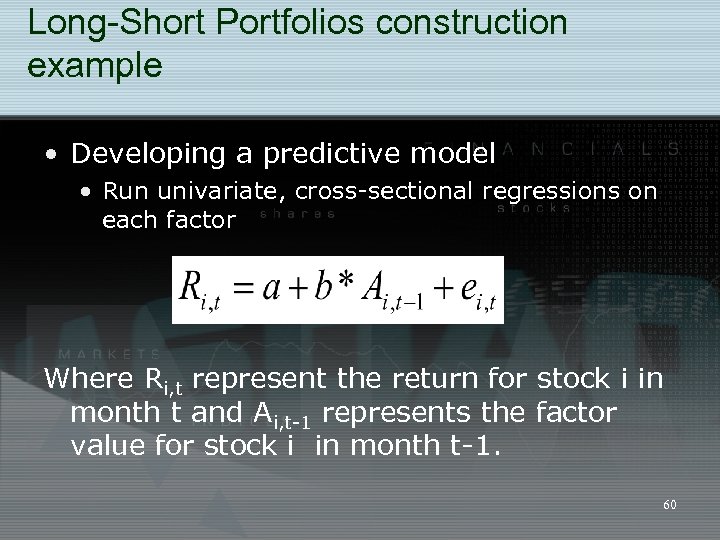Long-Short Portfolios construction example • Developing a predictive model • Run univariate, cross-sectional regressions on each factor Where Ri, t represent the return for stock i in month t and Ai, t-1 represents the factor value for stock i in month t-1. 60

Long-Short Portfolios construction example • We need to see how well our model works “out-of-sample”: • Run the regression model for years 1997 -2006. • Identify three factors that provide the greatest explanatory power (R 2) • Use the scoring screen method to select stocks to buy/sell during each month in 2007 • If factors do not work out-of-sample, they are not useful. 61

Long-Short Portfolios construction example • Here’s how it works…. • You select a set of 500 stocks (say S&P 500) • You determine that earnings yield, book to price and 1 year price momentum are most useful factors in explaining monthly returns. • for example, firms with high earnings yield in month t do exceptionally well in month t+1, firms with low earnings yield in month t do 62 poorly in month t +1.

Long-Short Portfolios construction example • Here’s how it works…. • Sort all the stocks by earnings yield. • For each of the 500 stocks, you assign a score of 3 (0, -3) if its earnings yield is in the top 100 (middle 300, bottom 100) each month. • You do the same for the other two factors. • Each stock will have a total score between 9 and 9. • The weights assigned to each factor can be altered, or determined by other variables. 63

Long-Short Portfolios construction example • Here’s how it works…. • Sort by total score • You purchase the top 50 or 100 stocks and you sell the bottom 50 or 100 stocks. • Repeat this procedure each month. • This is an example of a long-short portfolio where stocks are selected using a scoring screen. 64

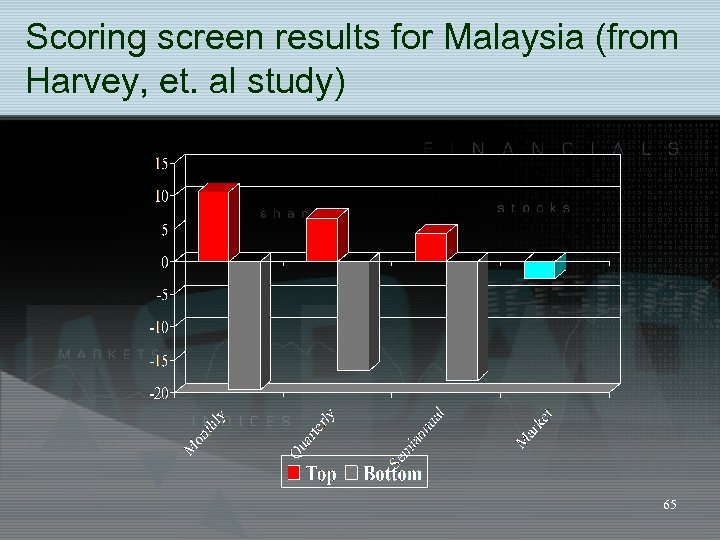Scoring screen results for Malaysia (from Harvey, et. al study) 65

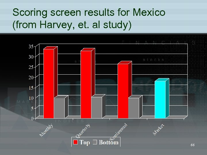Scoring screen results for Mexico (from Harvey, et. al study) 66

Technical analysis • What is technical analysis? • How can we combine this with fundamental analysis? • How do we read charts? • What are some of the commonly used technical tools and indicators? 67

Introduction • Technical analysis is the attempt to forecast stock prices on the basis of market-derived data. • Technicians (or quantitative analysts or chartists) are looking for trends and patterns in price and volume data that indicate future price movements. 68

Fusion Analysis • Practitioners and academics are more accepting of approaches that combine fundamental and technical analyses. These techniques are sometimes referred to as fusion analysis. • Fundamental analysis determines what securities to buy, technical analysis determines when to buy. • Another approach is to use technical analysis to identify groups or sectors, and fundamental analysis to pick stocks. 69

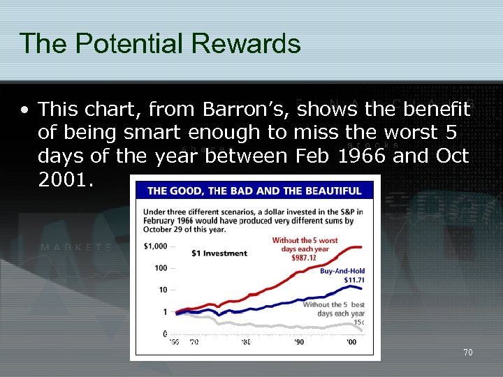The Potential Rewards • This chart, from Barron’s, shows the benefit of being smart enough to miss the worst 5 days of the year between Feb 1966 and Oct 2001. Source: “The Truth About Timing, ” by Jacqueline Doherty, Barron’s (November 5, 2001) 70

Charting • Chartists use bar charts or candlestick charts to look for patterns which may indicate future price movements. 71

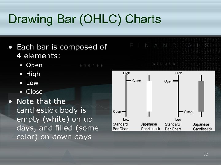Drawing Bar (OHLC) Charts • Each bar is composed of 4 elements: • • Open High Low Close • Note that the candlestick body is empty (white) on up days, and filled (some color) on down days 72

Trend lines • There are three basic kinds of trends: • An Up trend where prices are generally increasing. • A Down trend where prices are generally decreasing. • A Trading Range where prices are not moving substantially up or down. 73

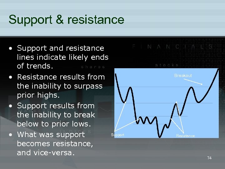Support & resistance • Support and resistance lines indicate likely ends of trends. • Resistance results from the inability to surpass prior highs. • Support results from the inability to break below to prior lows. Support • What was support becomes resistance, and vice-versa. Breakout Resistance 74

Moving averages • A simple moving average is the average price (usually the closing price) over the last N periods. • They are used to smooth out fluctuations of less than N periods. • An exponential moving average gives more weight to the most recent prices during the N periods. 75

Price patterns • Technicians look for many patterns in the historical time series of prices. • These patterns are reputed to provide information regarding the size and timing of subsequent price moves. 76

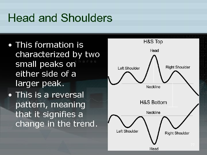Head and Shoulders • This formation is characterized by two small peaks on either side of a larger peak. • This is a reversal pattern, meaning that it signifies a change in the trend. 77

Technical Indicators • There are, literally, hundreds of technical indicators used to generate buy and sell signals. • We will look at three of the more commonly used indicators: • Moving Average Convergence/Divergence (MACD) • Relative Strength Index (RSI) • Accumulation/Distribution 78

MACD • MACD was developed by Gerald Appel as a way to keep track of a moving average crossover system. • Appel defined MACD as the difference between a 12 -day and 26 -day exponential moving averages. A 9 -day moving average of this difference is used to generate signals. • When this signal line goes from negative to positive, a buy signal is generated. • When the signal line goes from positive to negative, a sell signal is generated. • MACD is best used in choppy (trendless) markets. 79

Relative Strength Index (RSI) • RSI was developed by Welles Wilder as an oscillator to gauge overbought/oversold levels. • RSI is a rescaled measure of the ratio of average price changes on up days to average price changes on down days. • The most important thing to understand about RSI is that a level above 70 indicates a stock is overbought, and a level below 30 indicates that it is oversold (it can range from 0 to 100). 80

Accumulation/Distribution Line (volume indicator) • The Accumulation/Distribution Line was developed by Marc Chaikin to assess the cumulative flow of money into and out of a security. • The basic premise with this indicator is that volume precedes price. • Accumulation (distribution): when day’s closing price is higher (lower) than previous day’s close. • On accumulation (distribution) days the day’s volume is added (subtracted) from the previous days Acc/Dist line. 81

Accumulation/Distribution Line (volume indicator) • This indicator can be used to find situations in which the indicator is heading in the opposite direction as the price. • For example, downward price trend but upward Acc/Dist line would indicate that on up days volume is high, on down days, volume is low but there are more down days than up days. This suggests a reversal in price in the near term. 82

Readings • RB 6 • RB 16 (pgs. 606 - 612) • RM 4 83