Equilibrium Models with Interjurisdictional Sorting Presentation by Kaj

Equilibrium Models with Interjurisdictional Sorting Presentation by Kaj Thomsson October 5, 2004

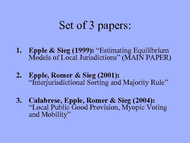
Set of 3 papers: 1. Epple & Sieg (1999): “Estimating Equilibrium Models of Local Jurisdictions” (MAIN PAPER) 2. Epple, Romer & Sieg (2001): “Interjurisdictional Sorting and Majority Rule” 3. Calabrese, Epple, Romer & Sieg (2004): “Local Public Good Provision, Myopic Voting and Mobility”

“Estimating Equilibrium Models of Local Jurisdictions” Dennis Epple Holger Sieg Journal of Political Economy, 1999

Background • Previously: Models characterizing equilibrium in system of jurisdictions (Tiebout models) • Assumption on preferences => strong predictions about sorting • Predictions not empirically tested

Basic framework (1): Setup • MSA = Set of Communities • Competitive housing market • price of housing determined by market in each community • Each community: 1 public good … financed by local housing tax

Basic framework (2): Equilbrium 1. Budgets balanced 2. Markets clear • • Housing markets Private goods markets 3. No household wants to change community (SORTING!)

Epple & Sieg (ES) test: 1. Predictions about distribution of households by income across communities 2. Whether the levels of public good provisions implied by estimated parameters can explain data

Formal Framework: • MSA with: • • Communities differ in: • • • C = continuum of households J communities Homogeneous land Tax on housing, t Price of housing, p ( p = (1+t)ph ) Households can buy as much housing as they want

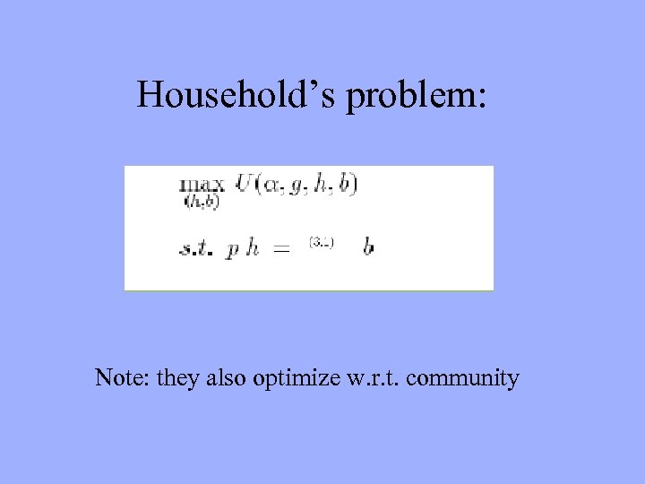
Household’s problem: Note: they also optimize w. r. t. community

Slope of indifference curve in the (g, p)-plane: • Assume: M( ) monotonic in y, α => • • Single-crossing in y (for given α) Single-crossing in α (for given y) …which is used to characterize equilibrium (A. 1)

What does single-crossing mean? • For given α, individuals with higher income y are willing to accept a greater house price increase to get a unit increase in level of public good

Also assume: 1. Agents are price-takers 2. Mobility is costless 3. Equilibrium existence - Shown in similar models - Found in computation examples … but not formally shown here

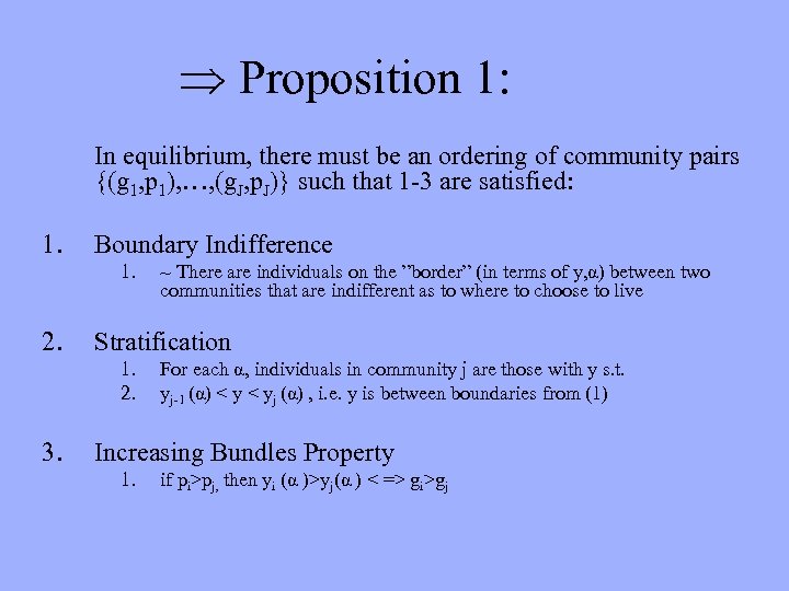
Þ Proposition 1: In equilibrium, there must be an ordering of community pairs {(g 1, p 1), …, (g. J, p. J)} such that 1 -3 are satisfied: 1. Boundary Indifference 1. 2. Stratification 1. 2. 3. ~ There are individuals on the ”border” (in terms of y, α) between two communities that are indifferent as to where to choose to live For each α, individuals in community j are those with y s. t. yj-1 (α) < yj (α) , i. e. y is between boundaries from (1) Increasing Bundles Property 1. if pi>pj, then yi (α )>yj(α ) < => gi>gj

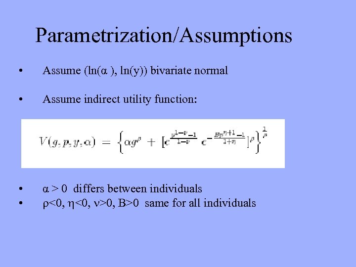
Parametrization/Assumptions • Assume (ln(α ), ln(y)) bivariate normal • Assume indirect utility function: • • α > 0 differs between individuals <0, >0, >0 same for all individuals

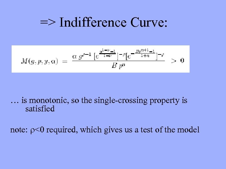
=> Indifference Curve: … is monotonic, so the single-crossing property is satisfied note: <0 required, which gives us a test of the model

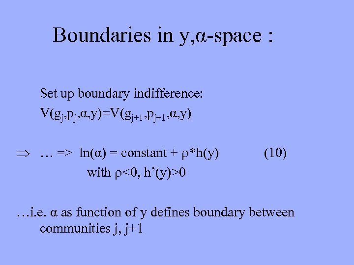
Boundaries in y, α-space : Set up boundary indifference: V(gj, pj, α, y)=V(gj+1, pj+1, α, y) Þ … => ln(α) = constant + *h(y) with <0, h’(y)>0 (10) …i. e. α as function of y defines boundary between communities j, j+1

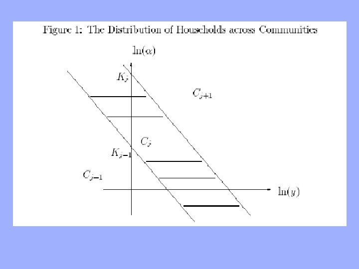
2 key results (& 3 Lemmas) 1. The population living in community j can be obtained by integrating between the boundary lines for community j-1 and j (L. 1) 2. We have system of equations (12) that can be solved recursively to obtain the communityspecific intercepts as functions of parameters (L. 2)

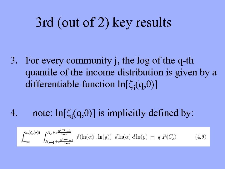
3 rd (out of 2) key results 3. For every community j, the log of the q-th quantile of the income distribution is given by a differentiable function ln[ i(q, θ)] 4. note: ln[ i(q, θ)] is implicitly defined by:

Summary (so far) Part III: Theoretical analysis => Equilibrium characteristics (Proposition 1) Part IV: Parametrization => computationally tractable characterizations (Lemma/results 1 -3) i. e. we now have a number of model predictions and we can test these predictions

Estimation Strategy Step 1: Match the quantiles predicted by the model with their empirical counterparts => identification of some parameters Step 2: Use the boundary indifference conditions => identification of the rest of the parameters

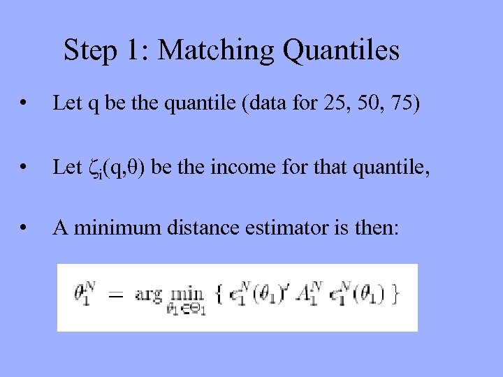
Step 1: Matching Quantiles • Let q be the quantile (data for 25, 50, 75) • Let i(q, θ) be the income for that quantile, • A minimum distance estimator is then:

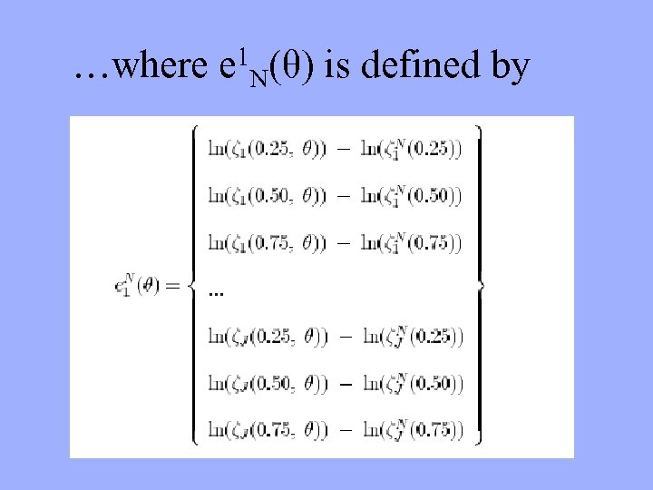
…where 1 e N(θ) is defined by

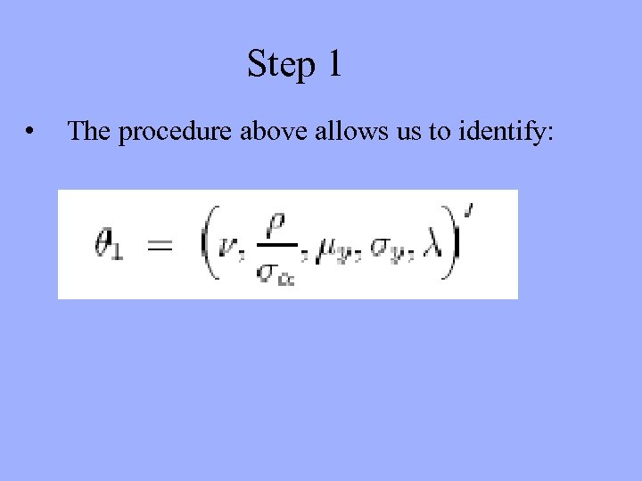
Step 1 • The procedure above allows us to identify:

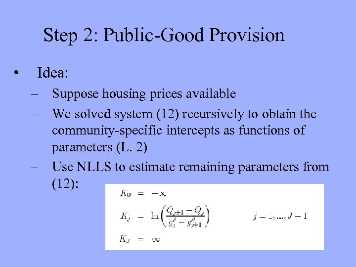
Step 2: Public-Good Provision • Idea: – Suppose housing prices available – We solved system (12) recursively to obtain the community-specific intercepts as functions of parameters (L. 2) – Use NLLS to estimate remaining parameters from (12):

Step 2: Public-Good Provision • Problem: • • (20) g enters system (12), but is not perfectly observed Solution: • • • Combine (12) and (20), and solve for j Can still use NLLS in similar way If endogeneity, find IV and use GMM instead of NLLS

Step 2 • The procedure above allows us to identify:

Data • • • Extract of 1980 Census Boston Metropolitan Area (BMA) 92 communities within BMA • Smallest: 1, 028 households (Carlisle) • Largest: 219, 000 (Boston) • Poorest: median income $11, 200 • Richest: median income $47, 646 … i. e. large variation

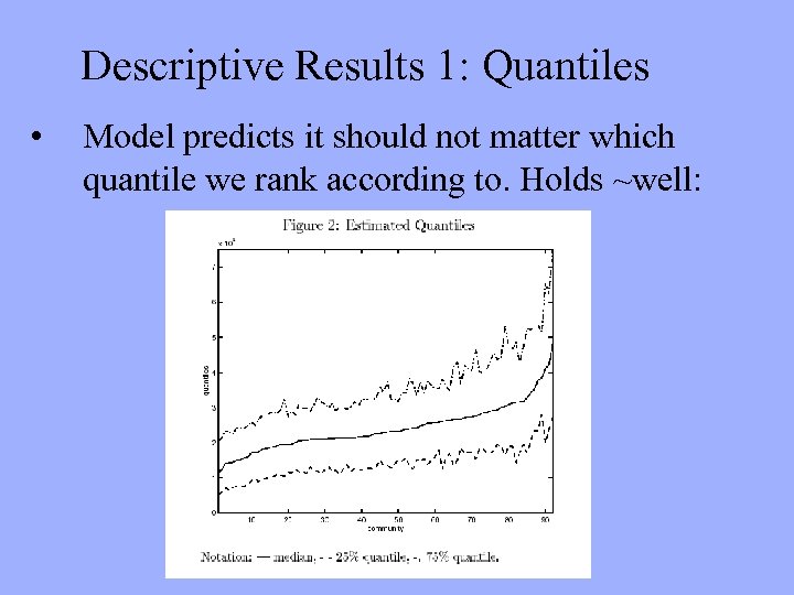
Descriptive Results 1: Quantiles • Model predicts it should not matter which quantile we rank according to. Holds ~well:

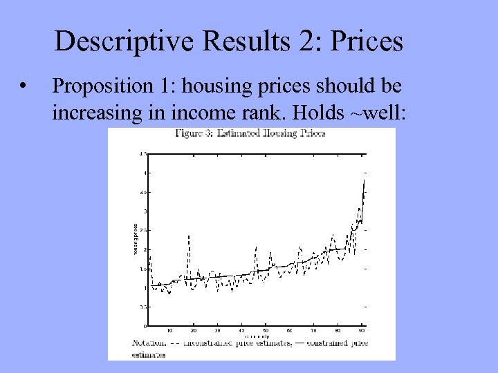
Descriptive Results 2: Prices • Proposition 1: housing prices should be increasing in income rank. Holds ~well:

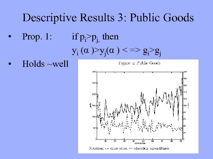
Descriptive Results 3: Public Goods • Prop. 1: • Holds ~well if pi>pj, then yi (α )>yj(α ) < => gi>gj

Some empirical results • In general, signs of parameter estimates compare well with empirical findings • Income sorting across communities important, but explains only small part of income variance • 89% of variance within community (heterogenous preferences) • Rich communities do provide higher levels of Public Goods (prediction supported)

Conclusions • What have we done? – – • Built structural model => set of predictions Checked predictions against descriptives (data) Estimated structural parameters Analyzed the parameters E & S: The structural model presented is able to replicate many of the empirical regularities we see in data

Comments (1) • Some assumptions questionable • • mobility costless? Can buy as much land as they want? • Single-crossing: Do they assume the implications/predictions of the model? • Evidence: Are the predictions really validaed? • What is the relevance of the model? Does it add anything to just looking at descriptive data

Comments (2) • … but still: • a nice ’exercise’ • shows that Tiebout models may have some predictive power (although says nothing about normative power, cf Bewley) • maybe the framework can lead to answers to policy relevant questions

The 2 Extensions Use the same framework, but … introduce voting behavior in communities: 1. Myopic Voting behavior 2. ”Utility-taking” framework 3. In general, mixed support for the models ability to predict and replicate data